PART I OF THE REPRESENTATION AND MEASUREMENTS OF URBAN TRANSPORTATION NETWORKS
Transportation modeling is at the core of urban transportation planning process. It attempts to simulate human behavior of travelling, estimates the impact of traffic on existing transportation networks, and provides reference for future infrastructure improvement, such as new roads or change of public transit system, for the next decades.
The conventional transportation modeling consists of four-step processes: trip generation, trip distribution, modal split and traffic assignment. First the target urban area is divided into tens or hundreds of traffic analysis zones (TAZs). Based on the socio-economic condition of each TAZ, the trips originated from each zone are generated as well as those destined for. The next step, trip distribution, constructs the estimated origin-destination (O-D) matrix. Take a study area of 100 TAZs for instance, a 100 x 100 O-D matrix will be established, where each cell in the matrix represents the total trips from one TAZ to another. This matrix will then be split, based on the choice of vehicle modes, into trips of car, bus or subway. In the last step, these trips are assigned to the roads in the real-world transportation network for the estimation of traffic flows, speed and capacity.
THE PROBLEM
A great number of variables are taken into consideration in this forecasting process which make the models and their calibration extremely sophisticated. Trip generation model uses population as well as school population, household numbers, income, car ownership, employment as key variables. A mysterious impedance function is created with distance and travelling cost in trip distribution model. Modal split model uses travel time value of different modes of vehicle, car maintenance cost, fuel charges, parking fees, etc. to construct the utility function of human-being. Traffic assignment establishes capacity restraint model of each travel mode to assign the trips to the real world network.
This study, consisting of a series of posts, will use the analysis methods and tools inspired by Social Network Analysis to offer an alternative angle of view on the urban transportation networks. This study will try to answer the question:
Where are the key nodes within the transportation network as well as those in greatest need of improvement?
Please note that this study is NOT for reviewing the conventional models or building a new one. This would require a large amount of data to provide a solid and complete review, which is far beyond the scope of this study.
THE METHODOLOGY AND ORGANIZATION OF THIS STUDY
Social Network Analysis (SNA) has been widely used in sociology, biology, information communication, etc. for decades. A network (or a graph) is established with a set of nodes and links (or edges) that connect them. SNA offers a collection of quantitative methods and tools to break into the networks and could provide valuable insights into urban transportation networks. Among various SNA methods, centrality is the most commonly used indicator to measure the importance of nodes within a network and identify the most influential one(s). While the study tries to solve the problem where the key traffic nodes are in the urban area, centrality serves as the best indicator throughout this series of posts.
There are several different types of centrality such as degree, closeness, betweenness and eigenvector centralities, each of them offering unique insights into the network. This study will discuss these centralities, their different ways of measurements and their strength and limitation in later sections.
The organization of this study is as follows:
1. Network representation and measurements of unweighted and undirected urban transportation networks
First, a network (or a set of nodes and edges to be more specific) of the study area is required to begin with before running any analysis. In part one, this study defines where these nodes are as well as what they represent for, and whether each two of the nodes exists a connection or not. Please note that the network created in this part is unweighted and undirected. This study then conducts the analysis with SNA tools and identify the key nodes in the network.
2. Welcome to the real world: assigning weights and directions to the network
The network structure in the real world is a lot different. The second part of this study assigns weights and directions to the nodes and edges of the transportation network so as to better represent the real world. Geocoding API provided by Google Maps Platform is used to calibrate the coordinates of the nodes; the weights and direction of edges are acquired by HERE Routing API; and the weights of nodes are assigned by using the socio-economic data of the study area.
3. Measurements of the weighted and directed network
Following part one and two, the third part of this study continues to use the SNA tools on the weighted and directed network to find the most important traffic nodes, edges and area in the real world. The results are also compared with those from part one.
4. Implications for urban transportation planning
This part focuses on answering the question asked in the beginning of the study with the findings from previous parts: to single out the traffic nodes and edges that are in the greatest need of improvement.
STUDY AREA
The study area includes the 456 lǐ’s (or urban villages/neighborhoods, the smallest unit of election administration in Taiwan) of Taipei City as nodes (or TAZs).
Previous studies of conventional transportation modeling in Greater Taipei Area (such as those conducted by Taipei Rapid Transit Corp.) usually covers not only Taipei City, but also New Taipei City, Keelung, and Taoyuan City. Qū’s (or districts, the upper administrative subdivision above villages) are used as TAZs in these studies. However, using villages as basic units of the study has the strength to look into more details in the network that will greatly improve the visualization of the research results and identify the whereabouts of the key nodes much more accurately. Moreover, the nodes’ coordinates on the map will significantly affect the weights assigned to edges and thus the results in the third part of the study, which is why villages, rather than districts, is a better and necessary choice.
Quick facts about Taipei City, Taiwan
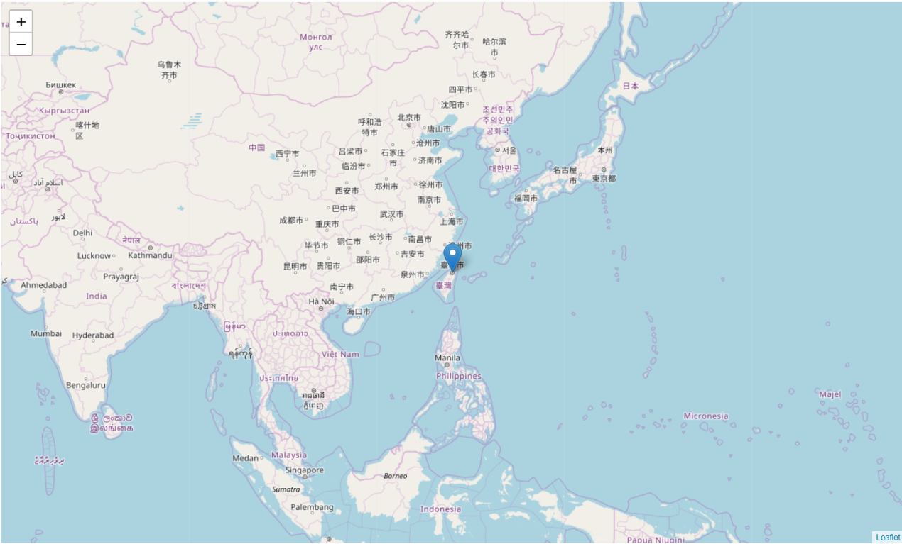
Taipei City locates in East Asia and is the political and socio-economic capital of Taiwan. Taipei City has a land area of 271.8 square kilometers (about the same size as Orlando, Florida), population of 2.6 million (close to the figure of Chicago), and a population density almost the same as New York City. The GDP (PPP) of Taipei City is estimated to be $300 billion, slightly higher than Atlanta, GA. Chinese Mandarin is the official language, which is why in the rest of this study you will see Chinese characters. This study will try to convert to English when necessary for better reading.
THE NETWORK PRESENTATION OF TAIPEI CITY
The Nodes: GeoJSON of Taipei Villages
In my previous study regarding accessible education resources, I used the GeoJSON file of Taipei contributed by littlebtc as the base map. This study continues to use the same GeoJSON file displaying the results. The GeoJSON file contains the polygon shapes of the 456 villages, each of them consisting of a set of coordinates that surround the polygon. The centroids of these polygons will serve as the nodes in the network in part one of this study. I’ll review and discuss further about the re-location of these nodes in the next part.
Below map shows the 456 villages on the map which you may interact with it(i.e. zoom in&out, click on the label, etc.).
The Edges: Connections between villages
After the base map and the 456 villages as nodes are created, the next step is to check all pairs of nodes to find out whether there’s a connection. This study defines an edge between two nodes exists if and only if the two polygons represented by the two nodes share at least one segment. More specifically, since each polygon is comprised of a set of coordinates, a shared segment simply means that there are at least two common coordinates in both polygons.
This study runs the checking on each polygon with the other 455 ones. Below table shows the result of connections from village no.0 to no.455. For example, village no.2 has connections with village no.1, 4, 6, 7, 8 and 19. Please note that these edges are undirected, that is, the total number of edges should be half the number showing in the table.
| NO |
village |
neighborhoods |
| 0 |
松山區莊敬里 |
[3, 4, 5, 8, 141, 143, 167, 327, 352] |
| 1 |
松山區東榮里 |
[2, 7, 8] |
| 2 |
松山區三民里 |
[1, 4, 6, 7, 8, 19] |
| 3 |
松山區新益里 |
[0, 4, 5] |
| 4 |
松山區富錦里 |
[0, 2, 3, 5, 6, 8] |
| 5 |
松山區新東里 |
[0, 3, 4, 6, 16, 17, 18, 349, 352] |
| … |
… |
… |
| 451 |
北投區關渡里 |
[386, 431, 450] |
| 452 |
北投區泉源里 |
[422, 439, 440, 442, 453, 454, 455] |
| 453 |
北投區湖山里 |
[404, 408, 409, 422, 452, 455] |
| 454 |
北投區大屯里 |
[442, 443, 445, 452, 455] |
| 455 |
北投區湖田里 |
[409, 452, 453, 454] |
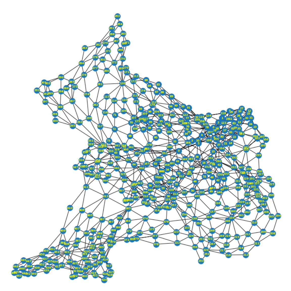
The basic representation of the urban network
Now with the nodes and edges, a network is presented. Below image is created with NetworkX to visualize this urban transportation network of Taipei City. NetworkX is a Python library for studying graphs and networks, which will be used in the next sections of this part of study. However such image is not intuitive for understanding the structure of the network.
I re-create the visualization of the network on the map (showing below), by locating the 456 nodes with their coordinates and connecting the nodes where an edge exists. This map helps find nodes and edges in a certain area more efficiently. Although the analysis results in the next sections won’t be any different whether to use a more friendly interface or not, this stduy hopes to provide another look at the network which brings better understanding for policy makers and for those who are interested.
NETWORK MEASUREMENTS (1): CENTRALITY
Centrality is useful in identifying the key nodes in a network and providing quantitative measures of the importance of the nodes so that these nodes can even be ranked. There are several different types of centrality, which measure and represent the “importance” in different aspects.
Degree Centrality
Degree centrality simply counts the number of edges each node has. A higher degree centrality means that the node links to more nodes. Below table shows the degree centralities of the top and bottom 10 nodes in the network, while the image shows how these nodes with different centralities distribute on the map. The bigger the nodes, the higher the degree centralities.
| |
Top10 |
c_degree |
Bottom10 |
c_degree |
| 0 |
北投區八仙里 |
0.0263736 |
萬華區榮德里 |
0.0043956 |
| 1 |
大安區學府里 |
0.0263736 |
萬華區柳鄉里 |
0.0043956 |
| 2 |
士林區福林里 |
0.0241758 |
文山區景美里 |
0.0043956 |
| 3 |
中山區集英里 |
0.021978 |
文山區試院里 |
0.0043956 |
| 4 |
南港區九如里 |
0.021978 |
文山區政大里 |
0.0043956 |
| 5 |
松山區精忠里 |
0.021978 |
士林區平等里 |
0.0043956 |
| 6 |
中山區大佳里 |
0.021978 |
大安區群英里 |
0.0043956 |
| 7 |
松山區莊敬里 |
0.0197802 |
南港區舊莊里 |
0.0043956 |
| 8 |
內湖區港墘里 |
0.0197802 |
信義區正和里 |
0.00659341 |
| 9 |
北投區建民里 |
0.0197802 |
士林區仁勇里 |
0.00659341 |
Despite the fact that degree centrality is relatively easy to understand, it is not a very good measure to identify the key transportation nodes in the real world, in that:
-
It only measures the number of nodes that one has direct connection with, which doesn’t provide any insights into the importance of the node within the entire network. For instance, a node with high degree centrality may not be an important traffic node if it is on the outskirts of the city.
-
The land areas of these 456 villages differ a lot. A bigger village could have a higher degree centrality simply because it shares segments with more smaller villages. Moreover, bigger villages are more likely in the peripheries of the city which could be hilly and inconvenient in traffic. In other words, a route may not exist between two adjacent villages in the real world. I’ll discuss more in detail in the second part of this study.
Closeness Centrality
Closeness centrality denotes the reciprocal of the sum of the shortest paths from one node to all other nodes in a network. Such definition is perhaps literally closest to the word “centrality”, like the geometric center. A node with higher closeness centrality has shorter average distance to all other nodes. This makes it a good indicator to a potentially good spot for regional logistics centers or emergency evacuates in the real world.
Below table shows the villages with the highest and lowest closeness centralities respectively. The network is also shown in the image, where the radius of a node represents its centrality value.
| |
Top10 |
c_closeness |
Bottom10 |
c_closeness |
| 0 |
中山區劍潭里 |
0.157005 |
萬華區榮德里 |
0.0717892 |
| 1 |
中山區大佳里 |
0.156411 |
萬華區銘德里 |
0.0753311 |
| 2 |
松山區莊敬里 |
0.154028 |
萬華區華中里 |
0.0772758 |
| 3 |
中山區新庄里 |
0.152072 |
萬華區錦德里 |
0.0779376 |
| 4 |
松山區精忠里 |
0.151717 |
萬華區孝德里 |
0.0793512 |
| 5 |
中山區圓山里 |
0.151414 |
北投區文化里 |
0.0805452 |
| 6 |
松山區中華里 |
0.14879 |
萬華區保德里 |
0.0813953 |
| 7 |
中山區集英里 |
0.147871 |
北投區智仁里 |
0.0817757 |
| 8 |
中山區成功里 |
0.146727 |
文山區景美里 |
0.0824873 |
| 9 |
松山區中正里 |
0.146491 |
北投區稻香里 |
0.0825172 |
Unsurprisingly, the nodes closer to the geometric center of the City have higher values of closeness centralities. However it’s worth noting that some nodes close to the east peripheries seem to have higher values than expected, forming some sort of “eastern corridor” that allows nodes to reach to others faster in an unweighted graph than in the real world. The existence of this “corridor” will be examined in the next part.
Betweenness Centrality
Betweenness centrality is arguably the most useful method in SNA to show the “traffic” happening within a network. To calculate the betweenness centrality, all shortest paths between every pair of nodes must be identified first. The betweenness centrality of a node is then defined as the times all shortest paths pass the node by. In other words, there are (456x455)/2 shortest paths among 456 nodes in Taipei transportation network. The highest-betweenness node means that it’s most likely to go through that village when moving in the city. That is, it has the most impact on the network if the node is removed from the network (or when the village is blocked somehow).
The top and bottom 10 villages are shown in below table. Below image illustrates the network where the radius of a node represents its value of centrality.
| |
Top10 |
c_betweenness |
Bottom10 |
c_betweenness |
| 0 |
中山區集英里 |
0.225073 |
士林區仁勇里 |
0 |
| 1 |
中山區劍潭里 |
0.209064 |
文山區景美里 |
0 |
| 2 |
中山區圓山里 |
0.200971 |
大安區群英里 |
0 |
| 3 |
中正區黎明里 |
0.200193 |
文山區明興里 |
0 |
| 4 |
中山區民安里 |
0.198732 |
文山區政大里 |
0 |
| 5 |
士林區福林里 |
0.18117 |
松山區新益里 |
0 |
| 6 |
松山區莊敬里 |
0.178926 |
南港區舊莊里 |
0 |
| 7 |
中山區大佳里 |
0.159007 |
文山區試院里 |
0 |
| 8 |
大安區學府里 |
0.150363 |
萬華區榮德里 |
4.84097e-06 |
| 9 |
中正區建國里 |
0.129745 |
北投區文林里 |
5.16371e-06 |
On the map there seems to exist two major pathways, one north-south and the other east-west, connecting the bigger nodes. Smaller nodes may move along branches to flow into the mainstreams (pathways) which allow them to move more quickly and efficiently to the destination in the network. Whether or not these pathway are present in the real world will be reviewed next.
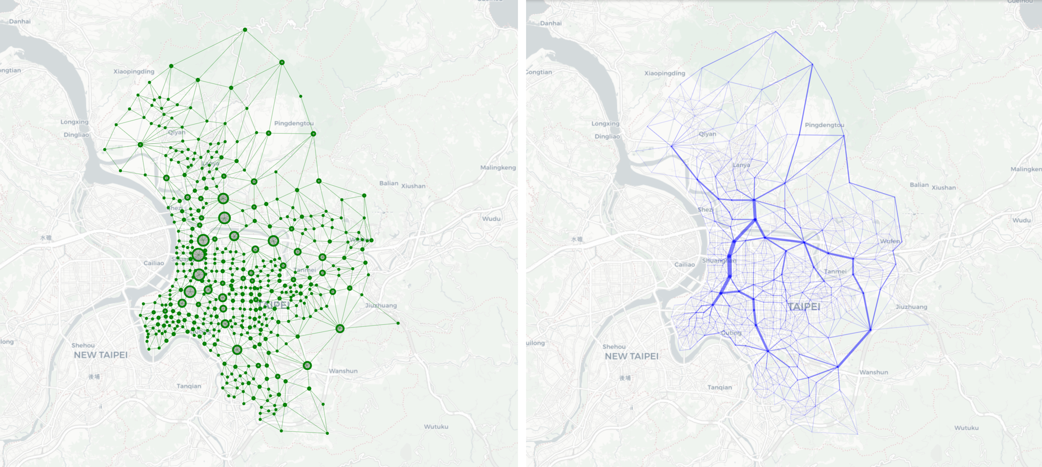
NETWORK MEASUREMENTS (2): EDGE BETWEENNESSES CENTRALITY
While the betweenness centrality shows the traffic passing through the nodes, the edge betweenness centrality, as suggested by its name, measures the traffic through the edges. Similar to the definition of betweenness centrality, edge betweenness counts the times all shortest paths between every pair of nodes in the network pass through that edge. The higher the edge betweenness, the more likely the edge will be used while moving from one node to another. In other words, if a high-betweenness edge is removed from the network, many shortest paths in the network will have to be re-routed.
Below table shows the edges (represented by two connected nodes) with the highest and lowest edge betweenness in the network. All edges are also shown in the image where thicker edges have higher betweenness.
| |
Top10_origin |
Top10_destination |
edge_betweenness |
| 0 |
中山區民安里 |
中山區集英里 |
0.191374 |
| 1 |
中山區集英里 |
中山區圓山里 |
0.182664 |
| 2 |
中山區民安里 |
中正區黎明里 |
0.146025 |
| 3 |
中山區劍潭里 |
士林區福林里 |
0.134018 |
| 4 |
中山區圓山里 |
中山區劍潭里 |
0.129222 |
| 5 |
中正區黎明里 |
中正區建國里 |
0.111785 |
| 6 |
大安區民炤里 |
大安區民輝里 |
0.0986036 |
| 7 |
南港區九如里 |
文山區博嘉里 |
0.098478 |
| 8 |
大安區龍門里 |
大安區學府里 |
0.0974406 |
| 9 |
中山區大佳里 |
中山區劍潭里 |
0.0971392 |
The map showing the edge betweenness centrality provides a more intuitive visualization of the transportation network in the real world. The above-mentioned north-south and east-west pathways into which smaller branches flow are better shown. Moreover, as discussed in the closeness centrality section, the “eastern corridor” that connects bigger villages along eastern peripheries is also clearer on the map. This explains why these nodes have higher centrality than expected, though it may not be the case in the real world.
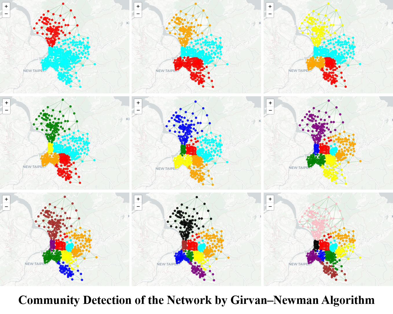
NETWORK MEASUREMENTS (3): COMMUNITIES
Community detection is one important study of SNA to understanding the structure of complex networks. A community is a set of nodes that connect to each other more densely internally than externally with another community. Community detection helps the understanding of the real-world transportation networks and the planning of the hierarchy of roads that link within local neighborhoods and between urban centers.
Several methods have been developed for finding communities within a network. However there’s no universal good algorithm that fits all needs. The number of communities, as well as how many nodes shall be contained, is usually unknown. Whether or not the communities shall overlap with one another also requires different methods. Nevertheless, the pros and cons of these algorithms are not in the scope of the discussion here.
This study uses the popular and widely-used Girvan–Newman algorithm for community detection. Though the method is often criticized for its terrible computation time O(m^2*n) which limits it to be adopted in a huge network analysis, for a network with 456 nodes it is still a decent choice. Another good reason for using the Girvan–Newman algorithm is that it continues the concept of edge betweenness centrality we’ve just discussed. First all edges’ betweenness centralities are calculated; the edge(s) that has the highest betweenness is removed from the network; the betweenness centralities of all those affected edges by the removal are then re-calculated; and finally this process continues to repeat until all edges are removed or the targeted number of communities are found.
The edges with high betweenness can be seen as “bridges” that connect different communities. Such “bridges” are more likely taken away first and the nodes from different communities will have to use another “bridge” to connect until there’s none. In other words, by gradually removing these bridges, the Girvan–Newman algorithm will finally isolate the communities from each other.
Below image shows the community detection process from when there are 2 communities to 12 different non-overlapping communities. The result provides a reference for the planning of the transportation hierarchy within and between the communities.
Comparing with the administrative districts in the real world
There are 12 districts in Taipei City, which is the reason I run the community detection process until there are 12 communities. Let’s see how they compare with each other. The left image below is the result from the Girvan–Newman algorithm, and the right shows the current districts.
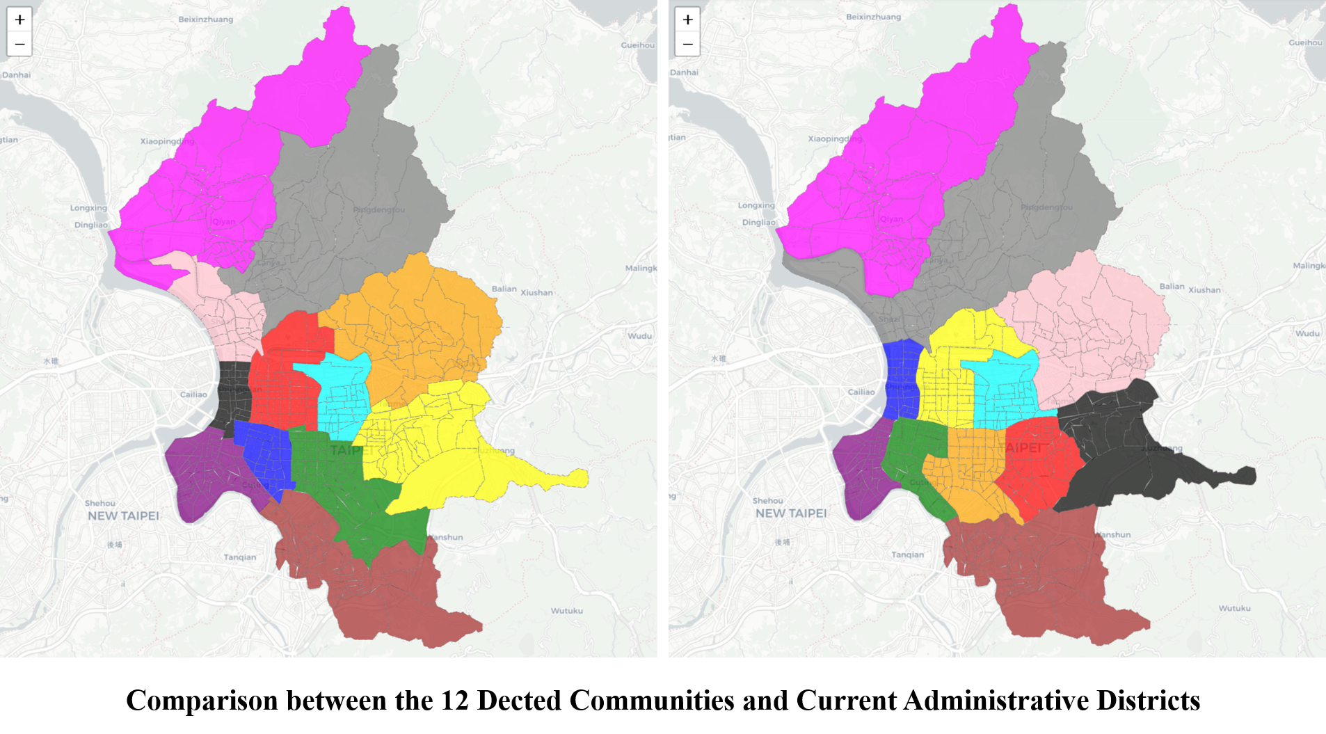
Despite the similarities of the communities/districts’ whereabouts shared between both images at a glance however, the result from the algorithm has one community less in the downtown than that from the actual districts (the blue, green and yellow from the left v.s. the green, orange, red and black from the right). Instead, one extra community is assigned to the pink area around western uptown.
The pink community called Siā-á from the algorithm is a peninsula area surrounded by rivers. Siā-á has been suffered from floods for a long time and is relatively isolated from the City. The algorithm interestingly detects this area as a community through the process.
SUMMARY OF PART ONE
This study provides an alternative perspective to look at the urban transportation network with a Social Network Analysis approach.
The first part of the study establishes an unweighted and undirected network of Taipei City. The centroids of the 456 lǐ’s (villages) are used to denote the nodes in the network, while edges are given if and only if any two villages’ polygons share at least one segment.
This study then uses SNA methods and tools on the network. Centrality is used to identify the key nodes in the network, which may indicates the important traffic zone in the real world; similarly the edges’ betweenness centrality are measured to find the potentially busy routes; and community detection algorithm groups nodes that are densely internal-connected, offering a reference to the planning of different levels of transportation within and between communities.
In the next part of this study, the urban transportation network will be reviewed and revised. Weights and directions will be defined and assigned to the nodes and edges. The location of the nodes will also be reviewed and updated with new coordinates so as to provide a better simulation of the real world.
SOURCE CODES
All source codes used in this post can be found on Colab or my GitHub.
INDEX