PART II OF THE REPRESENTATION AND MEASUREMENTS OF URBAN TRANSPORTATION NETWORKS
To better simulate the real world, this post reviews, defines and assigns the weights and directions to the network. The Geocoding API by Google Maps Platform as well as HERE Routing API are used to acquire the travel data.
PREVIOUSLY ON THE REPRESENTATION AND MEASUREMENTS OF URBAN TRANSPORTATION NETWORKS
In the first part of this study, an urban transportation network of Taipei City is established, by using the centroids of 456 lǐ’s (aka villages) as the nodes and the connections between two adjacent villages as the edges. A preliminary analysis is then conducted with Social Network Analysis (SNA) methods and tools. Centrality is used to identify key nodes and edges in the network, and community detection is used to provide a reference for the planning of the hierarchy of roads within and between the communities.
This network is unweighted and undirected, and therefore has its limitation, such as:
- The unweighted edges doesn’t reflect the traffic (e.g. distance, time, cost) in the real world;
- Going back and forth between two locations may take different routes and thus different time or distance, which is not represented in an undirected network;
- Villages have different number of residents, commercial facilities and companies, which would generate or attract trips that differ a great deal; and
- An edge may not even exist between two adjacent villages. For example, two villages separated by rivers may not directly link to each other; and there may be no route to connect those in the hilly peripheral areas.
In this post, these problems will be addressed and resolved by defining and assigning the weights and directions to the network.
THE WEIGHTS OF THE NODES
Description
Traffic is the flows of human activities. The conventional transportation model estimates the trips generated and attracted by each Traffic Analysis Zone (TAZs) by using various socio-economic data as variables. For example, the generation of work trips requires household number, number of workers in the household, persons in an age group, household income, etc. while the attraction needs the number of employees, floor area of establishment, etc. In a sophisticated model each TAZ should have at least two different variables to represent its generation of trips as the origin and attraction as the destination.
Having said that, this study uses the population of residents, a more generalized variable, to represent the weights of the nodes in the network. Later in Part Four of this study, more data would be reviewed and used to reflect more specific situations of the real world and to revise the network if necessary.
Data Acquisition
The population of all villages in the end of 2019 is acquired on the website of Taipei City Government. Below table shows that the average population of a village is 5,800, ranging from the minimum 939 to the maximum 11,836. This huge difference in population would reflect on the trips generated from the villages.
| |
total_ppl |
| count |
456 |
| mean |
5800.53 |
| std |
2049.63 |
| min |
939 |
| 25% |
4429.25 |
| 50% |
5611.5 |
| 75% |
7123.5 |
| max |
11836 |
Below image shows the population of all the villages on the map where bigger nodes have more residents. It’s worth noting that the population of villages in the peripheral areas is not necessarily fewer than those in the center of the city, given that the land area is also bigger.
RELOCATION OF THE NODES
Description
In order to adopt an SNA approach, the nodes are used to represent the villages instead of polygons. In Part One of this study, the geometric centroids are used to denote the nodes of the network on the map. However, the analysis results on this unweighted and undirected network is not affected by the location of the nodes. In fact, it doesn’t matter if a map is used or not. Visualization of the results on the map is for better understanding only. Having said that, when it comes to assigning weights and directions to the network, the location of the nodes will have significant impact on the weights of the edges.
To resolve this issue, one solution is to increase the number of nodes (TAZs). I’ve replaced the 12 districts commonly used in the conventional model with 456 villages which largely improves the representation of nodes for the villages in the real world. However, there is still room for improvement.
A geometric centroid is a decent choice to represent a village when the land area is small enough and the population is distributed more evenly. Here there are still exceptions that need to be taken care of, where the centroids may locate in a river, a zoo, the National Park, the airport, or simply in the middle of nowhere. There’s one centroid not even located within the village because of its unique shape. In these cases, centroids can be misleading.
A solution is to find a better location to represent the node of the TAZ. Given that the traffic flow comes from human activities, the choice shall be the spot where most population resides, or where the people have best access to.
Vote with feet, literally!
In this study, the location of village offices is used as the new nodes to replace geometric centroids. Villages are the smallest electoral units in Taiwan. The elected chiefs’ duty is to reflect the public opinions, help enhance the awareness of policies, and organize and host social events. For those who seek for the re-election every four years, a good service is most crucial and therefore their offices are always located at the most convenient spots where residents can access to. In other words, the residents can literally vote with their feet for a candidate who better serves their needs by simply being closer to their lives, in the very first step.
Data Acquisition and Wrangling
This study collects the location of the village offices by acquiring the addresses from the Taipei City Government, showing below.
| |
dist |
neigh |
姓名 |
里辦公處電話 |
手機 |
address |
| 1 |
松山區 |
莊敬里 |
劉美鳳 |
2.76068e+07 |
0920309000 |
撫遠街369巷12號1樓 |
| 2 |
松山區 |
東榮里 |
鄭玉梅 |
2.76769e+07 |
0933902948 |
民生東路5段69巷3號1樓 |
| 3 |
松山區 |
三民里 |
謝翠鈴 |
2.76714e+07 |
0910380103 |
民生東路5段163-1號8樓 |
| 4 |
松山區 |
新益里 |
吳美貞 |
8.78776e+07 |
0936841566 |
富錦街581巷20號 |
| 5 |
松山區 |
富錦里 |
李煥中 |
2.76382e+07 |
0912546233 |
富錦街515號 |
| … |
… |
… |
… |
… |
… |
… |
| 452 |
北投區 |
中和里 |
黃景煌 |
2.89422e+07 |
0919210306 |
中和街365號 |
| 453 |
北投區 |
大屯里 |
張天恩 |
2.89118e+07 |
0985325333 |
復興三路521巷18號 |
| 454 |
北投區 |
智仁里 |
傅書淵 |
2.89653e+07 |
0933764271 |
杏林二路74巷3號 |
| 455 |
北投區 |
秀山里 |
陳壽彭 |
2.89417e+07 |
0937022555 |
中和街502巷2弄15號 |
| 456 |
北投區 |
文化里 |
周世英 |
2.89175e+07 |
0952914338 |
文化三路55號1樓 |
The next step is to convert the addresses to geographic coordinates, a process which the Geolocation API by Google Maps Platform is exactly designed for. Below table shows the results returned from Geocoding API, the latitudes and longitudes as well as the formatted addresses in English for all villages. There are 458 rows of results, which implies that there exists duplicates to be removed. One missing data is to be amended, too.
Below image shows where these coordinates are located on the map. Obviously not all the results are correct. There are at least two spots far from where they are supposed to be. Geocoding API always returns the most alike results which may be incorrect in some cases if there are no perfect matches for the requested addresses.
The results returned from the Geocoding API are checked where they actually locate, and cross-compare with where they are ought to be. The comparison (below table) shows that 14 sets of coordinates are not within the villages they represent. Two of them are not even in Taipei City, as also shown in above map.
| |
dist_neigh |
office_address |
office_loc |
| 24 |
松山區中正里 |
台北市長安東路3段229號12樓 |
中山區興亞里 |
| 31 |
松山區福成里 |
台北市敦化南路1段100巷6號2樓A室 |
大安區德安里 |
| 43 |
信義區五常里 |
台北市永吉路225巷7弄34號2樓 |
信義區四育里 |
| 76 |
大安區龍安里 |
台北市和平東路1段199巷4-9號 |
NA |
| 119 |
大安區群英里 |
台北市四維路198巷30弄9號1樓 |
大安區群賢里 |
| 128 |
中山區正得里 |
台北市中山北路1段135巷40號3樓 |
中山區中山里 |
| 193 |
中正區幸福里 |
台北市北平東路24號 |
中正區梅花里 |
| 224 |
萬華區福星里 |
台北市西寧南路14之3號1樓 |
萬華區萬壽里 |
| 237 |
萬華區糖廍里 |
台北市大理街106號1樓 |
萬華區糖蔀里 |
| 248 |
萬華區銘德里 |
台北市長泰街219號1樓 |
萬華區保德里 |
| 375 |
士林區明勝里 |
台北市承德路4段5之1號 |
士林區後港里 |
| 400 |
士林區天和里 |
台北市中山北路7段154巷6號4樓(天母區民活動中心) |
士林區天山里 |
| 426 |
北投區吉利里 |
台北市石牌路1段39巷120弄7號 |
北投區尊賢里 |
| 446 |
北投區湖山里 |
台北市湖山路1段48之2號 |
NA |
One by one the addresses of these 14 village offices are examined on their official websites. While nine sets of the coordinates are found wrong and need to be corrected, two offices are indeed located within other villages, two on the borderline of the GeoJSON shapes which happen to be assigned to the other village, and the final one is a typo so that it cannot be matched. The updated location of the village offices are shown below.
Comparing Village Offices’ Location with Geometric Centroids
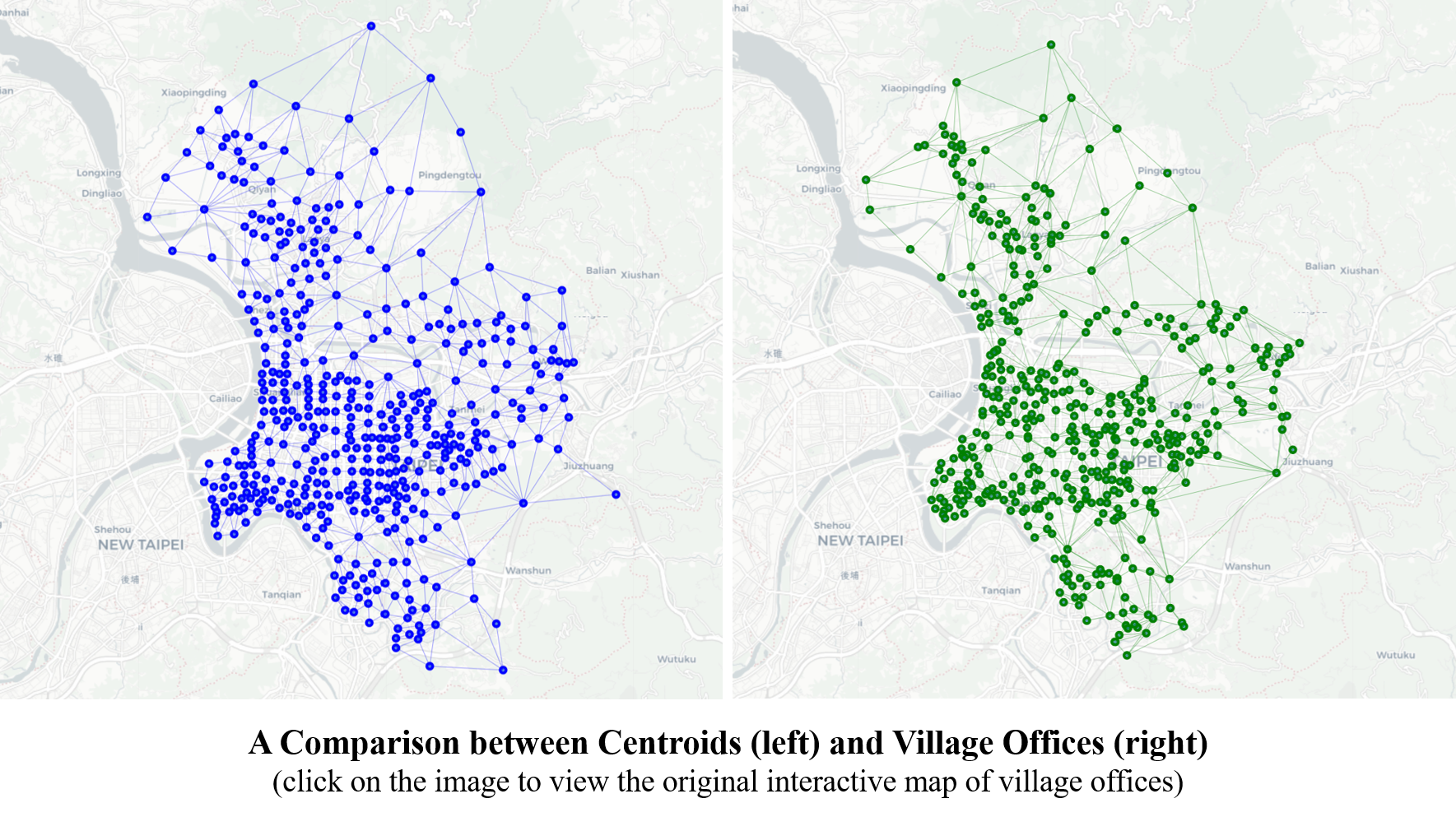
Below images show a comparison between the location of the nodes by using centroids (left) and the coordinates of the village offices (right). Significant differences are found that:
- The nodes representing the peripheral village offices are more inward and closer to the center of the City.
- The centroids distribute more evenly and are more separated from one another, while the offices tend to concentrate either along the main roads or in the residential area, leaving out more “blank areas”. These areas could be riverbanks, the airport, an university, a military base or Government buildings.
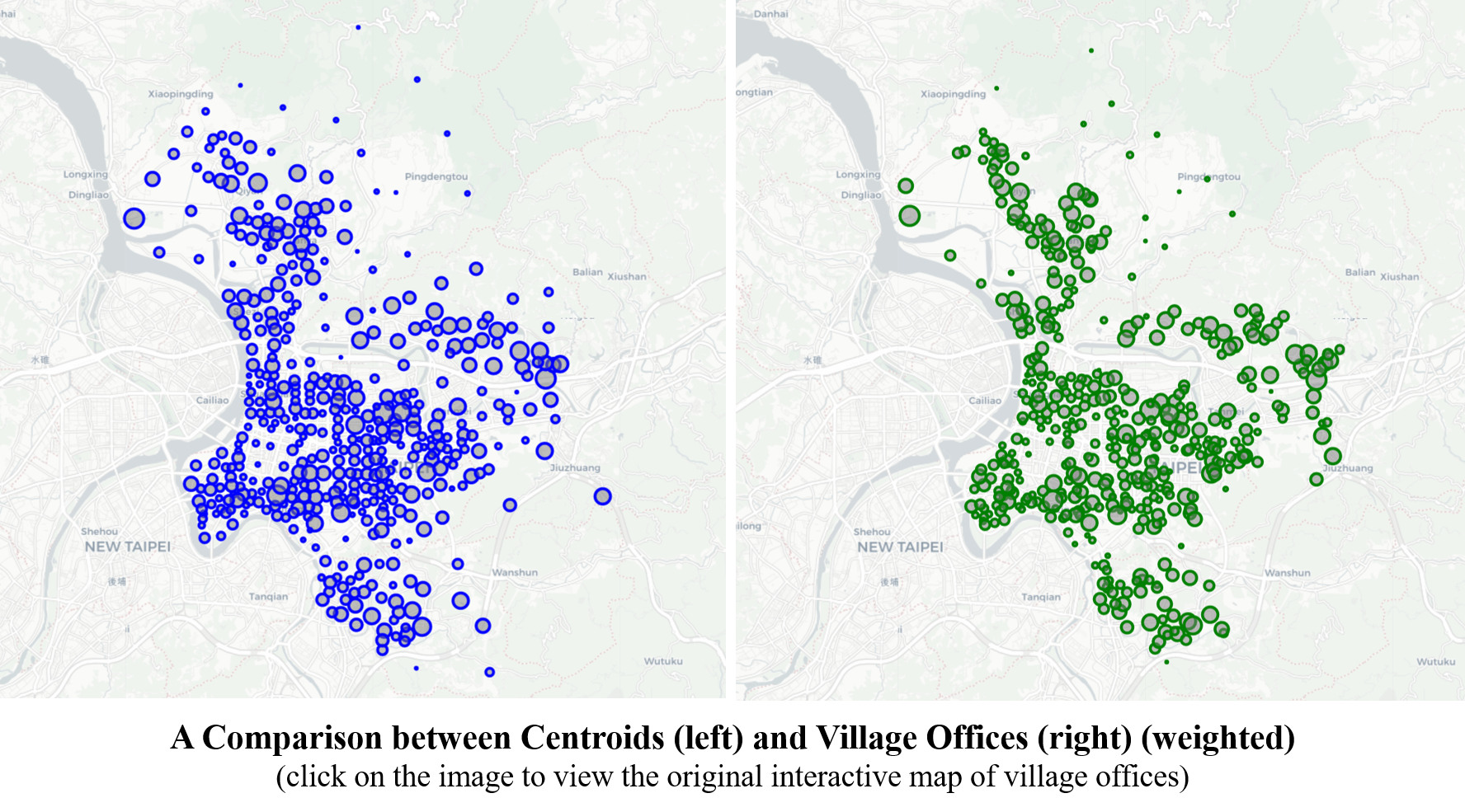
Adding weights of the nodes to the images gives the idea how the population actually resides in the City. The above-mentioned points are also clearer. In the up-town, most offices distribute along a corridor; in the mid-town, the airport and the riverbanks are left out; and in the down-town, the nodes are more concentrated, avoiding the land of universities, Central Government as well as Taipei City Government buildings.
The Limitation
In a transportation network, directions shall also be considered and given to the nodes.
In this section, the coordinates of village offices are used to denote the nodes. Comparing to the geometric centroids, the village offices can better identify where most population reside within the villages or where villagers can access most conveniently. In other words, the offices’ location is a good choice to represent the residents where the trips are generated from, that is, the origin. Having said that, the offices may not serve as an equally good choice as a destination. More specifically, take work trips for instance, the employees working in the destination village will need to be studied. A node has to be chosen to represent the workplaces such as an industrial zone or government office building, instead of the village office or the geometric centroid. Similarly, all kinds of schools need to be taken into account when analyzing the school trips.
In this study I focus on a more generalized transportation network. The different purposes of trips are not considered here. However, both weights and directions (as an origin and a destination) of nodes will need to be reviewed and assigned when conducting further studies of any specific purpose of trips.
THE WEIGHTS AND DIRECTIONS OF THE EDGES
Description
In the conventional transportation forecasting model, the trips between every pair of TAZs (the O-D matrix) as the dependent variable are estimated. The variables used in the model include the properties of the TAZs (such as the population, employment and number of schools) as well as the properties of the connections between each TAZ (such as distances, traffic time and cost).
In this study the shortest traffic time (which is why the location of nodes matters) between each pair of villages is used to represent the weights and directions of the edges, in that:
- The traffic time reflects the accessibility between two nodes;
- The traffic time can also represent the cost to some extent; and
- The traffic time changes during peak hours and off-peak hours, which provides insights into where the traffic is worse and in need of immediate improvement.
Among different modes of transport such as car, bus, subway and bike, the travel time could differ a lot, not to mention that one of the most commonly-used vehicle in Taiwan is motorcycle, which is not widely covered in researches.
This study focuses on only one kind of vehicles, car, to continue the rest of the study. Please bare in mind that the results of the study cannot be overexplained to any other kind of vehicles.
Data Acquisition
HERE Routing API is used in this study to acquire the traffic time. Majority-owned by automotive companies including Audi, BMW and Daimler, HERE provides services such as maps, geolocation and navigation. Their clients include Garmin, Alpine and Amazon.
A Routing API request can be customized with very detailed condition set out by users to fit their own needs, including:
- Routing Type allows users to search the fastest route with the least amount of travel time, or the shortest route that returns the least amount of distance. This study uses the fastest routing type so that the time difference between rush hours and off-peak hours can be directly compared. Please note that in the rest of this study, the shortest path(s) will be refer to as the route with the shortest travel time, unless otherwise specified.
- Transport Mode provides routing choices for car, bicycle, public transport and pedestrians, where car is used for later study.
- Traffic Mode specifies whether to optimize a route for traffic. It provides real-time traffic closures and speed is used if road would be traversed during travel. Since the purpose of the study is to compare how the traffic becomes during peak hours, the traffic mode is enabled.
- Departure and Arrival Time allow users to set out the time when the travel is expected to start/end. Traffic speed and incidents are taken into account when calculating routes. To observe the impact of peak hours, this study set the arrival time to be 8:30 in the morning during weekdays.
- Response Data Types return several attributes such as a summary (including overall route distance and time), the shape of route as a polyline, legs of route, maneuver group that provides itinerary summary and brief route instructions, etc. Travel time in summary and the route shape will be used for later study.
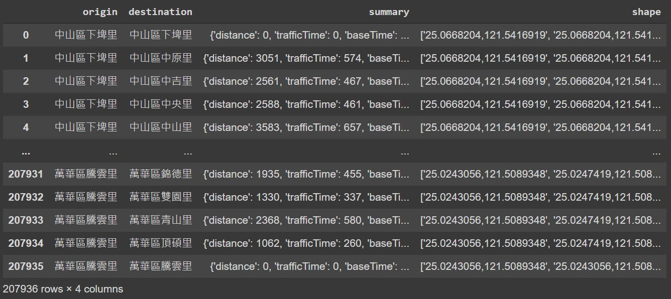
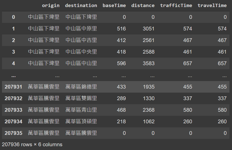
Using the 456 nodes as both start and end waypoints, this study acquires more than 200,000 routes (456 times 456) between all pairs of nodes. Below table shows the origin and destination of each route and the summary of response data from HERE Routing API as well as the shape of the route.
Data Wrangling (1): Travel Time
Four attributes of a route are given in the summary. Expanding the summary of the 207,936 routes gets the table below. TrafficTime and BaseTime both contain the travel time estimate in seconds, where TrafficTime considers traffic conditions while BaseTime not. TravelTime is the same as TrafficTime when the Traffic mode is set as enabled. Distance indicates the total travel distance for the route, in meters.
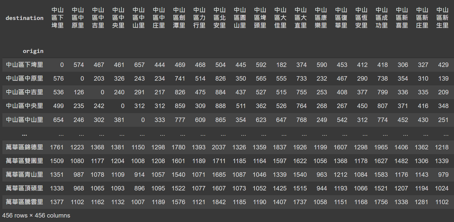
A 456x456 O-D matrix is constructed by rearranging the travel time of all routes, showing below. Each row represents the travel time needed from one specific village to all other 455 villages.
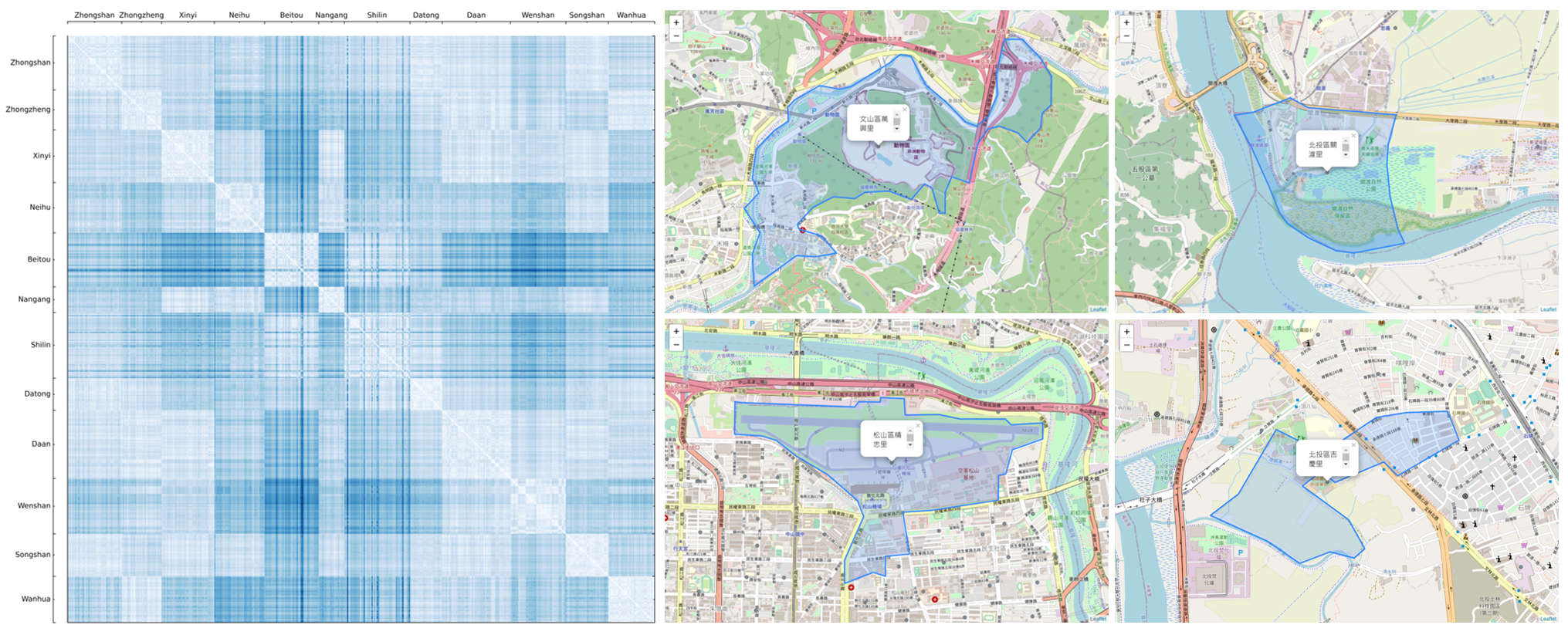
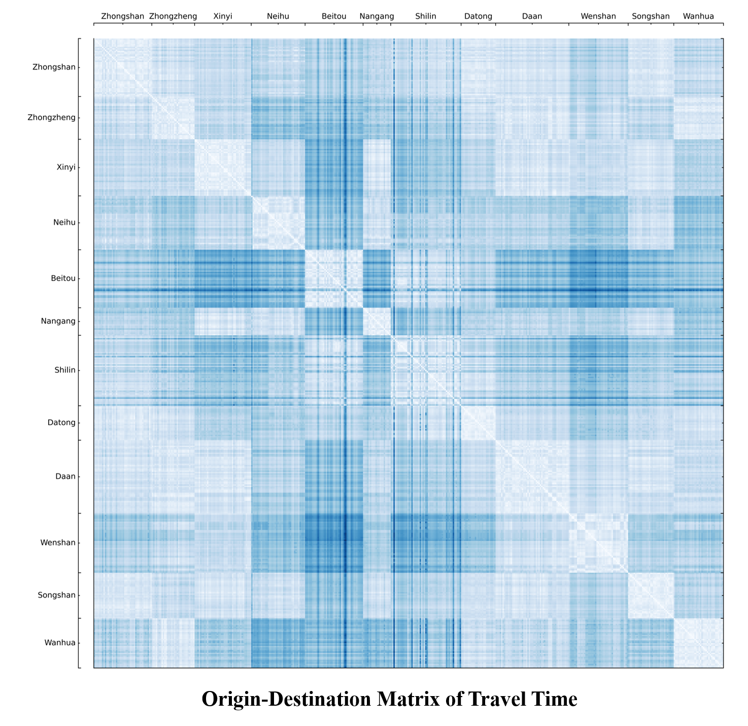
Below image is the visualization of the O-D matrix. The color in each cell represents the travel time, which gets darker when the travel time gets longer. Meanwhile the 456 villages are grouped by the districts (the upper administrative unit) they belong to. As can be told from the image, districts such as Beitou, Wanhua and Wenshan are more distant districts that have longer travel time to other districts. Please note that this image does not imply whether the traffic is worsen during rush hours. The traffic condition will be further discussed in Part Four of this study.
Data Wrangling (2): Traffic Routes
Based on request conditions, HERE Routing API returns the routes with the least traveling time. The exact route is contained within the response datatype shape as a polyline, which consists of a set of coordinates. Below image shows an example of 455 routes originated from one village only. Without doubt there are lots of duplicated legs of routes which will be used to proceed the SNA methods in the third part of this study.
Checking the routes originated from the nodes confirms the concerns brought out in the beginning of the study:
1. A connection may not exist between two adjacent villages, that is, the shortest path needs to go through yet another village(s). Below image shows all shortest routes originated from one northeastern village. This node has 6 edges in the unweighted and undirected network. However, in real world it relies on only one route to connect with the rest of the network. Such situation is also found in other peripheral nodes as well as those close to a river.
2. The shortest path may take routes beyond the scope of the City. In the routes map originated from one southwestern village showing below, an expressway provides a shorter path connecting to other peripheral villages. This study will discuss more in detail about the calculation of SNA tools in the next part.
SUMMARY OF PART TWO
Part One of this study builds an unweighted and undirected transportation network and performs preliminary study with SNA methods and tools. To better simulate the real world, this part defines and assigns the weights and directions to nodes and edges.
The weight of a node is defined as the number of residents in the village, which reflects traffic flows originated by human activities. The location of the village offices are used to represent the nodes, in replace of the geometric centroids, in that the village office has the best accessibility within the village and thus is a better choice than a centroid.
The weight and direction of an edge is defined as the traffic time between two nodes, which reflects the accessibility and travel cost. The traffic time difference between peak hours and off-peak hours will also be used to provide a reference for transportation improvement in future. In this study, car is used as the vehicle for the calculation of the traffic time.
In next part of this study, the SNA methods and tools will be used to analyze this weighted directed network.
SOURCE CODES
All source codes used in this post can be found on Colab or my GitHub.
INDEX