PART III-(1) OF THE REPRESENTATION AND MEASUREMENTS OF URBAN TRANSPORTATION NETWORKS
This post first examines Closeness Centrality of the real-world network, and points out potentially highest accessible villages in the City. Though not widely covered in any studies, nodes’ weight is also taken into consideration to look at the service coverage problem. The groups of villages that cover a certain amount of population within a given travel time are then identified.
PREVIOUSLY ON THE REPRESENTATION AND MEASUREMENTS OF URBAN TRANSPORTATION NETWORKS
Part I of this study establishes a transportation network of Taipei City. The 456 villages are used to denote the nodes and an edge between two nodes exists only when the villages share a segment of the boundary. SNA tools and measurements, such as centrality and community detection, are then used to conduct a preliminary study on this unweighted and undirected network.
The second part reviews, defines, measures and assigns the weights and directions of the nodes and edges in the network, so as to better simulate the real-world transportation network. The weight of a node is defined as the population living in the village, and the geolocation is also calibrated, moving from the geographic centroid to the coordinates of the village office. Travel time is used to denote the weight and direction of the edges.
In this part of study, the SNA methods will be used to study this weighted, directed network. The results will be compared with those in the first part. This post focuses on closeness centrality first. The definition and how to calculate using real-world data will be elaborated more in detail.
DEFINITION OF CLOSENESS CENTRALITY IN REAL WORLD
Closeness centrality of a node denotes the reciprocal of the average shortest paths between that node and all other nodes in a network. It can be represented by the below equation:
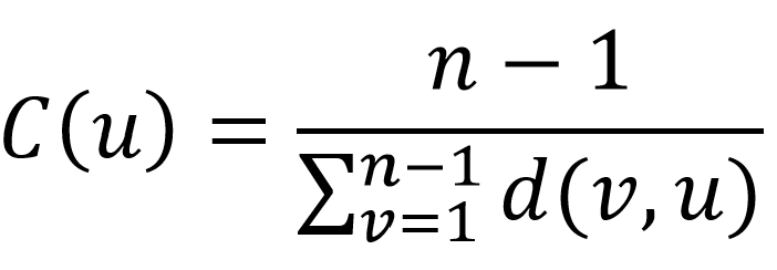
where C(u) is the closeness centrality of node u; n is number of nodes; and d(v ,u) is the shortest-path distance between node u and node v.
In an unweighted network, the distance between any two connected nodes is set as one. The distance between node u and v is therefore the number of edges of the shortest path. Below image is the closeness centrality of the unweighted Taipei transportation network from Part I of the study, with nodes resized by closeness score.
In real world, the shortest-path distance can have different definitions such as the linear distance between two nodes’ geo-coordinates or the distance of the travel route by some specific vehicle. However the physical distance does not change from time to time and cannot reflect the traffic condition. Since the main focus of this study is looking for insights into the improvement of the transportation network, the distance is therefore not a good measure for closeness centrality here.
As a result, this study denotes the shortest path by travel time, in that the travel time, like distance, indicates how far it is between two nodes and, unlike distance, it could also differ a lot during peak and off-peak hours, reflecting dynamic traffic condition in the network.
DATA
In the second part of this study, the travel time data is retrieved using HERE Routing API. Below 456x456 O-D matrix shows the travel time between all pairs of the 456 villages, that is, the weights of edges.
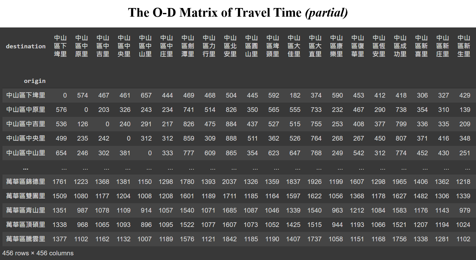
Note that these edges have directions. The travel time from node A to node B is not necessarily equal to that from node B to A. This study will calculate the closeness centrality of each node of 2 two different directions, respectively. The outward closeness of a node uses the travel time from that node towards all other nodes, while the inward closeness accounts for the travel time arriving from all nodes. That is, the outward closeness will sum up the travel time of each row in above matrix (and then take the reciprocal of the average travel time) where the villages serve as the origin. Similarly, the outward closeness sums up the travel time of each column where the villages are destinations.
RESULTS
Inward and Outward Closeness Centrality of the Real World
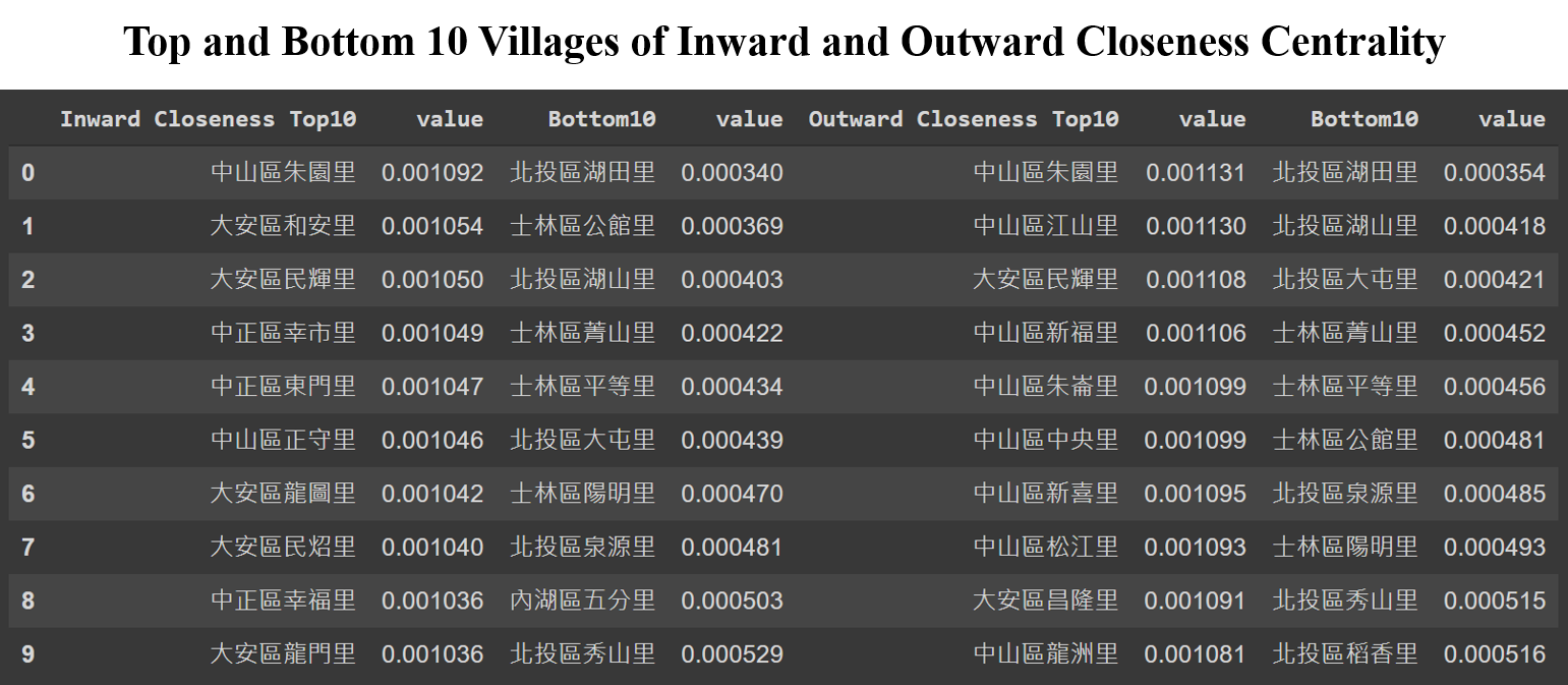
Using the travel time provided in the O-D matrix, below table shows the top and bottom 10 villages ranking by inward and outward closeness centrality, respectively. By definition, the villages with higher inward closeness are more accessible from anywhere within the City, while travelling from villages with higher outward closeness takes fewer time to reach all other villages.
Below images show the inward (up) and outward (down) closeness on the map where nodes with a high closeness degree are enlarged. These two images share a lot in common: high-closeness nodes concentrate in-between the mid- and down-town, while peripheral nodes especially those from far uptown are the more distant from the network, for both getting into and out from.
Comparison with the Unweighted Network
Below image shows the comparison of closeness between that derived above and that calculated from the unweighted, undirected network in Part One. For better reading and understanding, the nodes and edges view is replaced by the zonal view, where each polygon represents the village’s geographical boundary and the color darkens with higher score.
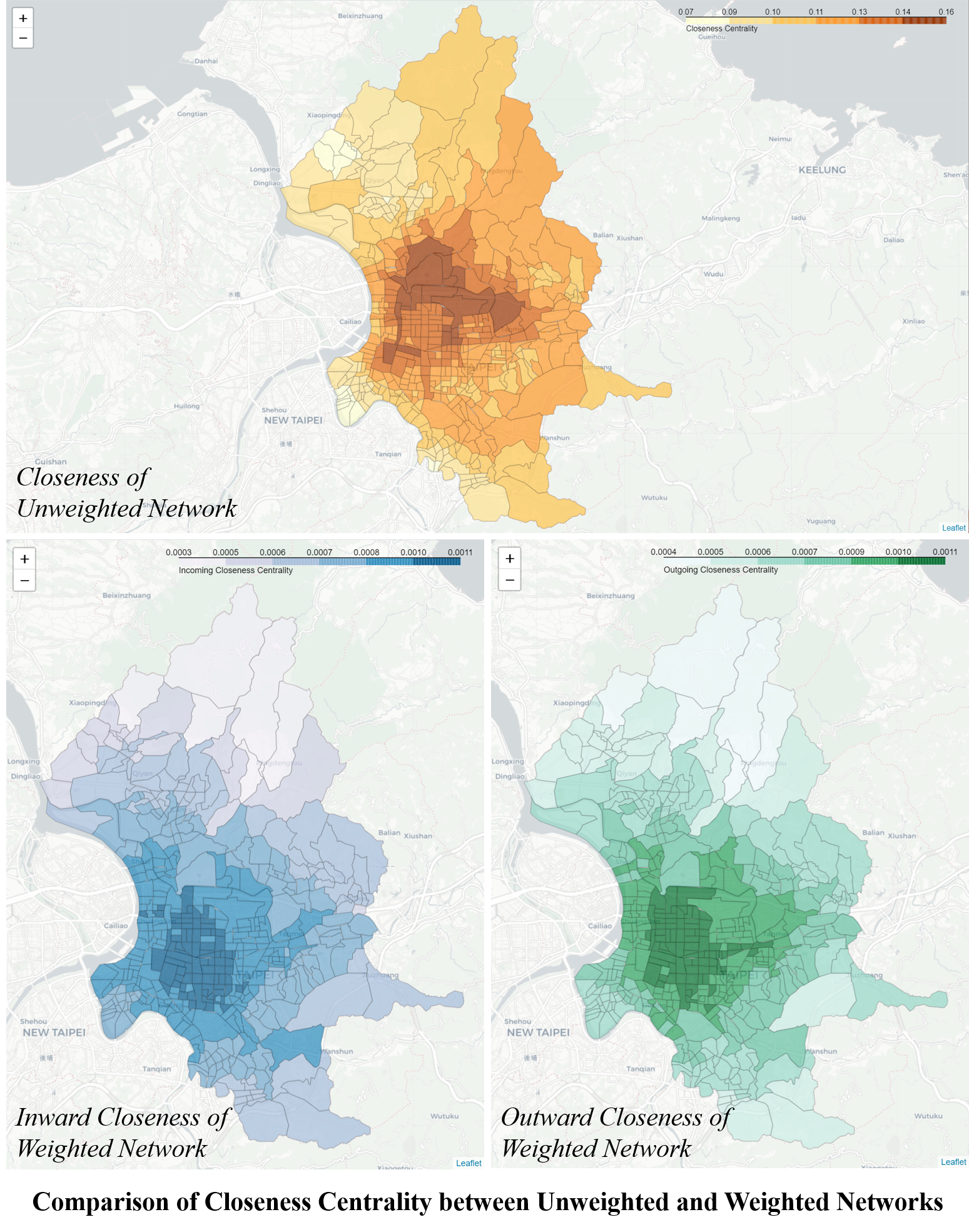
While, in the real world network, villages with higher inward and/or outward closeness concentrate in the southwestern part of mid-town, those high-score villages in the unweighted network tend to distribute in the northern part of the mid-town and are generally bigger in land area. These bigger villages have more connections with others which gives them the advantage to serve as a corridor collectively, providing a shorter path to connect villages from one end to the other in the unweighted network. However, in real world these villages are usually separated by the river, the airport or the military base, which makes them not as well connected as it seems to be.
In the weighted, directed network, the area where high-score villages locate is the old town of Taipei City, where expressways, from south to north as well as from east to west, intersect. This fact makes the area much more accessible to and from anywhere in the City, which also reflects on the higher values of both inward and outward closeness.
TAKING NODES’ WEIGHTS INTO ACCOUNT
Closeness centrality has been used to check on both weighted and unweighted networks so far. However in a weighted network, the closeness measure considers only weights (and directions) of edges, but not weights of nodes. Theoretically the nodes’ weights will not affect the measurement of closeness centrality, given that the the value of a node is defined in terms of shortest path distance or time to/from other nodes, and has nothing to do with the node itself.
Having said that, the study of the closeness centrality can still be extended according to the research topic to provide meaningful findings. In this section, the nodes’ weight is defined as the population of the villages. Inward closeness centrality will be used to discuss the ideal nodes for installing collection center(s) and their service coverage areas, while the outward closeness is for discussion of installing distribution centers.
Inward Closeness and In-Reachable Population
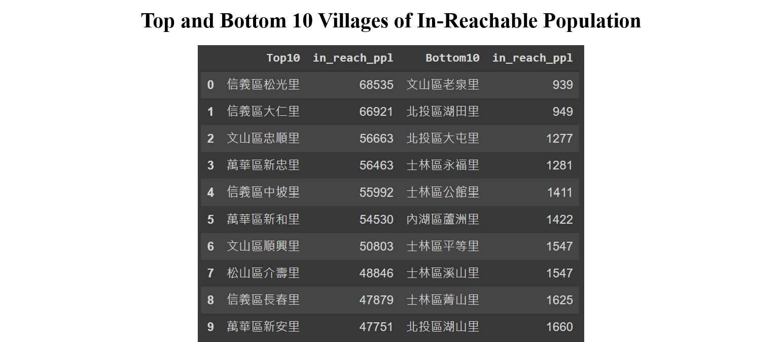
Using the measures of inward closeness of each node and the village population as its weight derives the total population arriving from the reachable area within a given time. A node with higher reachable population means that more people can arrive at the location of the node within time, which makes it a good choice as a logistics collection center, or an emergency evacuation spot.
The in-reachability ranking of nodes will look a lot different given different search conditions. Below table shows the top & bottom 10 villages and their covered population within 3-minute travel time by car. The covered population ranges from less than one thousand to almost 70K. It’s worth noting that the covered area of the top villages might be duplicated simply because they are small and close to one another. For example, the highest in-reachable village “信義區松光里” covers a population of 68,535 from 11 villages, including 3 other villages in top10 (No. 2, 5 and 9).
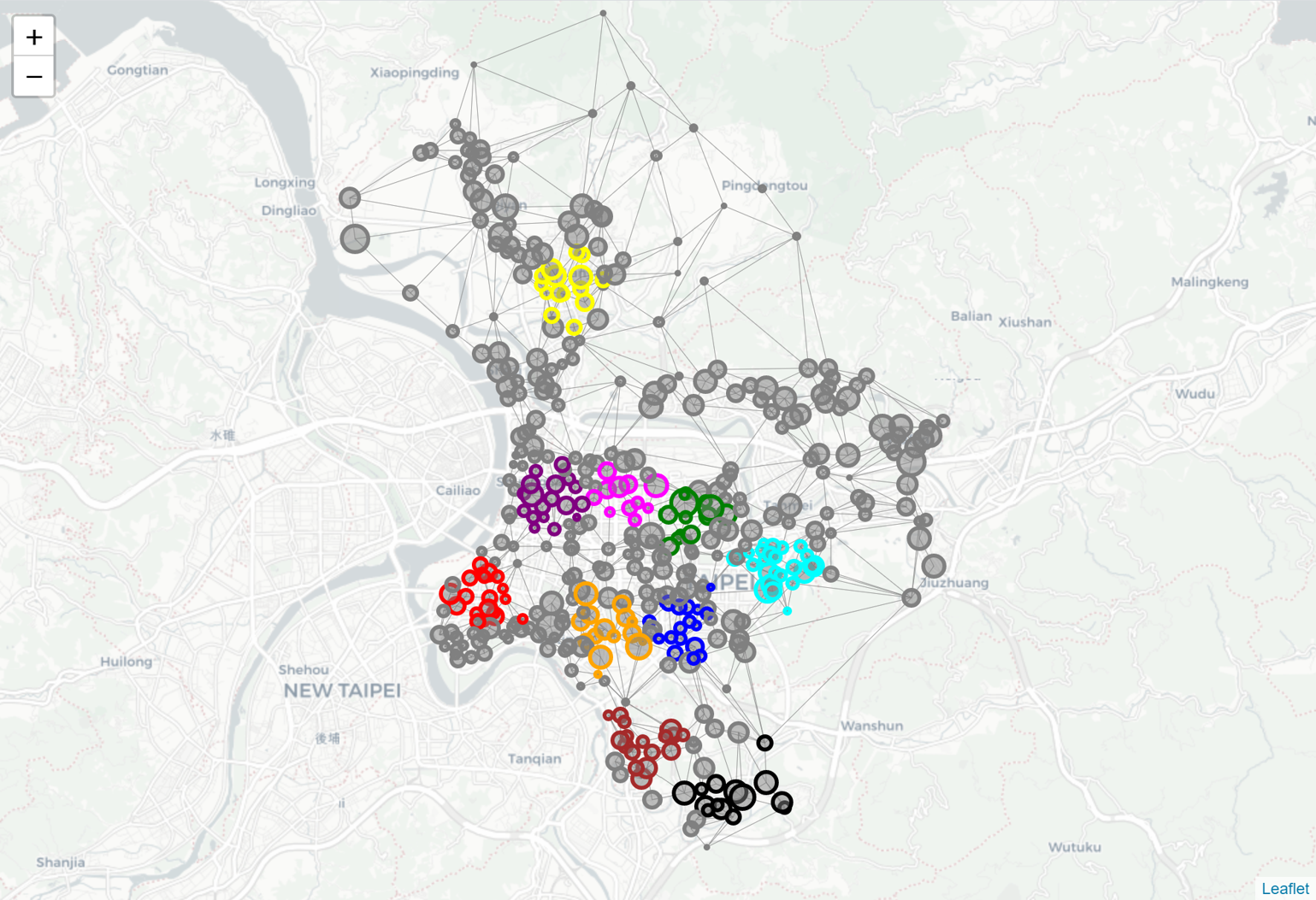
Searching all nodes that cover at least 40K population within 3 minutes and grouping the nodes with their covered nodes, the result shows that only 8 groups satisfy the condition. Below image shows these 8 groups in different colors with the nodes resized by the population.
The condition can be changed depending on the research topic. The number of groups may increase when travel time increases or the covered population decreases. Likewise, the number of groups decreases the other way around.
Below image shows the change of the distribution where the highest in-reachable villages locate when the travel time increases. Within 10 minutes, there are still some high score villages found in different local areas of the City. However, these villages quickly get concentrated in the southwestern part of the mid-town after 10 minutes, the same as the distribution of inward closeness described in previous section.
Outward Closeness and Out-Reachable Population
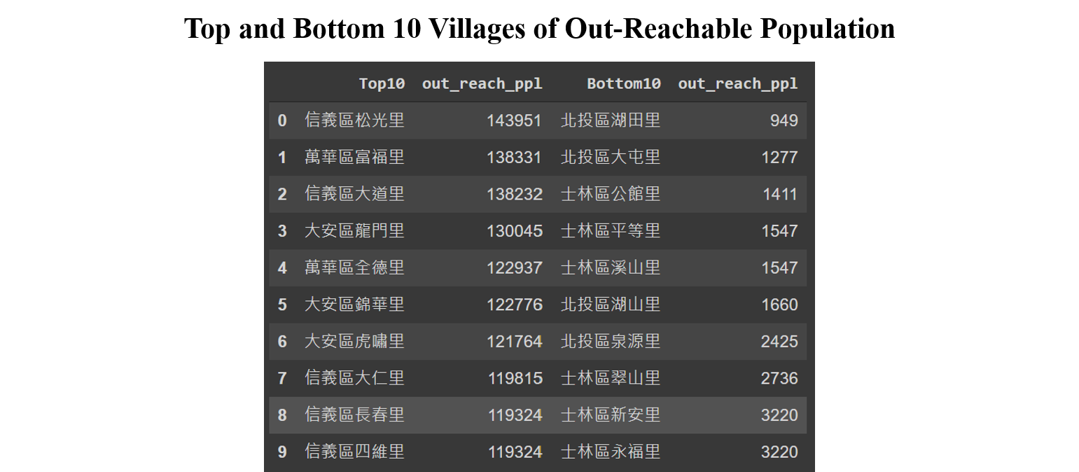
Replacing the inward closeness with the outward shows the out-reachable population from each node within travel time. A node with more out-reachable population means that more people can be approached from the location of the node, making it suitable for a logistics distribution center, a command center, or a popular food delivery service spot.
Top and last 10 villages and their reachable population are shown in below table. The highest score village covers a population of almost 150K.
Setting out-reachable population of 100K within 5 minutes as the search condition, 10 villages and their covered villages are shown in below image. Please note that these groups have prevented duplicated nodes to be shown in two or more groups.
Below image shows the change of villages’ out-reachable population when travel time increases. Similarly to that of in-reachable population, the high score villages can be found in different areas in the City within 10 minutes, which then concentrate in the midtown area after that.
SUMMARY OF PART III (1)
This post uses the SNA closeness centrality measure to run the analysis on the real world network. The inward closeness of a node implies the accessibility from the network toward that node, while the outward closeness means the other way around. A node with high inward closeness measure is good for a logistics collection center, and similarly a high-outward node is suitable for distribution center.
This post further uses the population as the nodes’ weight to look in detail at the service coverage problem. Given different service coverage conditions, that is, a certain population within a certain travel time, this post shows that different groups of villages can be found within the City.
In the next post of Part III, this study will continue the analysis on the other vital SNA tool – betweenness centrality, which is arguably the best measure and indicator to reflect the traffic condition of the real world. By using the travel routes retrieved in Part II, next post will show the likelihood of each node and edge being used when travelling in the network, that is, the potential higher traffic areas that may need immediate improvement.
SOURCE CODES
All source codes used in this post can be found on Colab or my GitHub.
INDEX