PART IV-(1) OF THE REPRESENTATION AND MEASUREMENTS OF URBAN TRANSPORTATION NETWORKS
The travel-time delay of all 207,936 routes, 456 villages and 2,070 edges within the network of the City is calculated, visualized and discussed. This post identifies the villages as well as the edges with relatively bad traffic condition during morning peak time.
PREVIOUSLY ON THE REPRESENTATION AND MEASUREMENTS OF URBAN TRANSPORTATION NETWORKS
So far I’ve examined Taipei transportation network, both weighted and unweighted, with the social network analysis tools. In the last post, betweenness centraility has been introduced for identifying the nodes and edges most likely to pass by when travelling in the City, which make potentially critical areas of traffic conflicts. However, are these the areas in need of immediate improvement or investment in infrastructure? To answer this question, at least two factors have to be brought into consideration: how many people are travelling through the specific nodes and edges and how bad is the traffic?
First let’s examine the traffic status within the network in the first post of Part IV of this study.
THE MEASUREMENT OF THE TRAFFIC CONDITION
The reason why traffic condition needs to be addressed here is because the betweenness centrality simply means the probability of usage of a node or edge, and is not necessarily equal to the sufficiency or satisfactory of the traffic. In other words, there may already exist state-of-the-art infrastructure in the busiest zones to cope with the traffic impact during rush hours. In the traffic assignment (or route choice) process of the conventional transportation modelling, various factors such as the number of lanes and the width of the roads are taken into the model for the calculation of the capacity of the roads.
This study uses the travel-time delay during the morning peak time as the indicator to whether the infrastructure is overloaded. The worse the time delayed, the more prior an improvement is needed.
TRAVEL-TIME DELAY OF ROUTES
In Part II of the study, HERE Routing API is used to acquire the shortest routes between all pairs of the 456 villages. HERE also provides the information of the travel time, including both the traffic time (that considers traffic speed) and the base time that neglects the traffic conditions. With these two elements, the travel-time delay is derived. The base time, traffic time as well as the travel-time delay of the 456x456 routes are shown in below table.
| |
origin |
destination |
baseTime |
trafficTime |
delay |
| 0 |
Xiabi Vil. |
Xiabi Vil. |
0 |
0 |
0 |
| 1 |
Xiabi Vil. |
Zhongyuan Vil. |
516 |
574 |
0.112 |
| 2 |
Xiabi Vil. |
Zhongji Vil. |
412 |
467 |
0.133 |
| 3 |
Xiabi Vil. |
Zhongyang Vil. |
418 |
461 |
0.103 |
| 4 |
Xiabi Vil. |
Zhongshan Vil. |
596 |
657 |
0.102 |
| … |
… |
… |
… |
… |
… |
| 207931 |
Tengyun Vil. |
Jinde Vil. |
433 |
455 |
0.051 |
| 207932 |
Tengyun Vil. |
Shuangyuan Vil. |
289 |
337 |
0.166 |
| 207933 |
Tengyun Vil. |
Qingshan Vil. |
468 |
580 |
0.239 |
| 207934 |
Tengyun Vil. |
Dingshuo Vil. |
218 |
260 |
0.193 |
| 207935 |
Tengyun Vil. |
Tengyun Vil. |
0 |
0 |
0 |
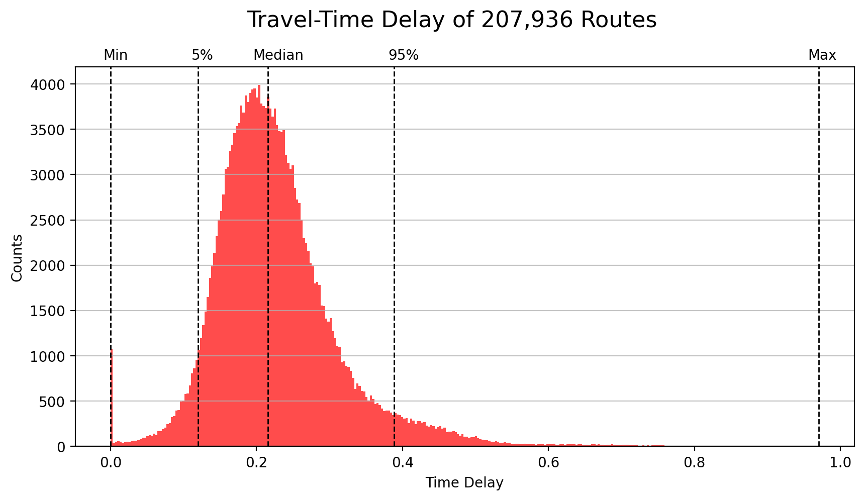
Below figure illustrates the frequency distribution of travel-time delay of these 207,936 routes. Most routes have the delay time between 0.12 and 0.38, meaning that travelling during peak hours would take 12% to 38% more time. Note that this distribution is right-skewed and have a very long tail. Some routes have much worse travel-time delay and would take almost double time to complete the trip.
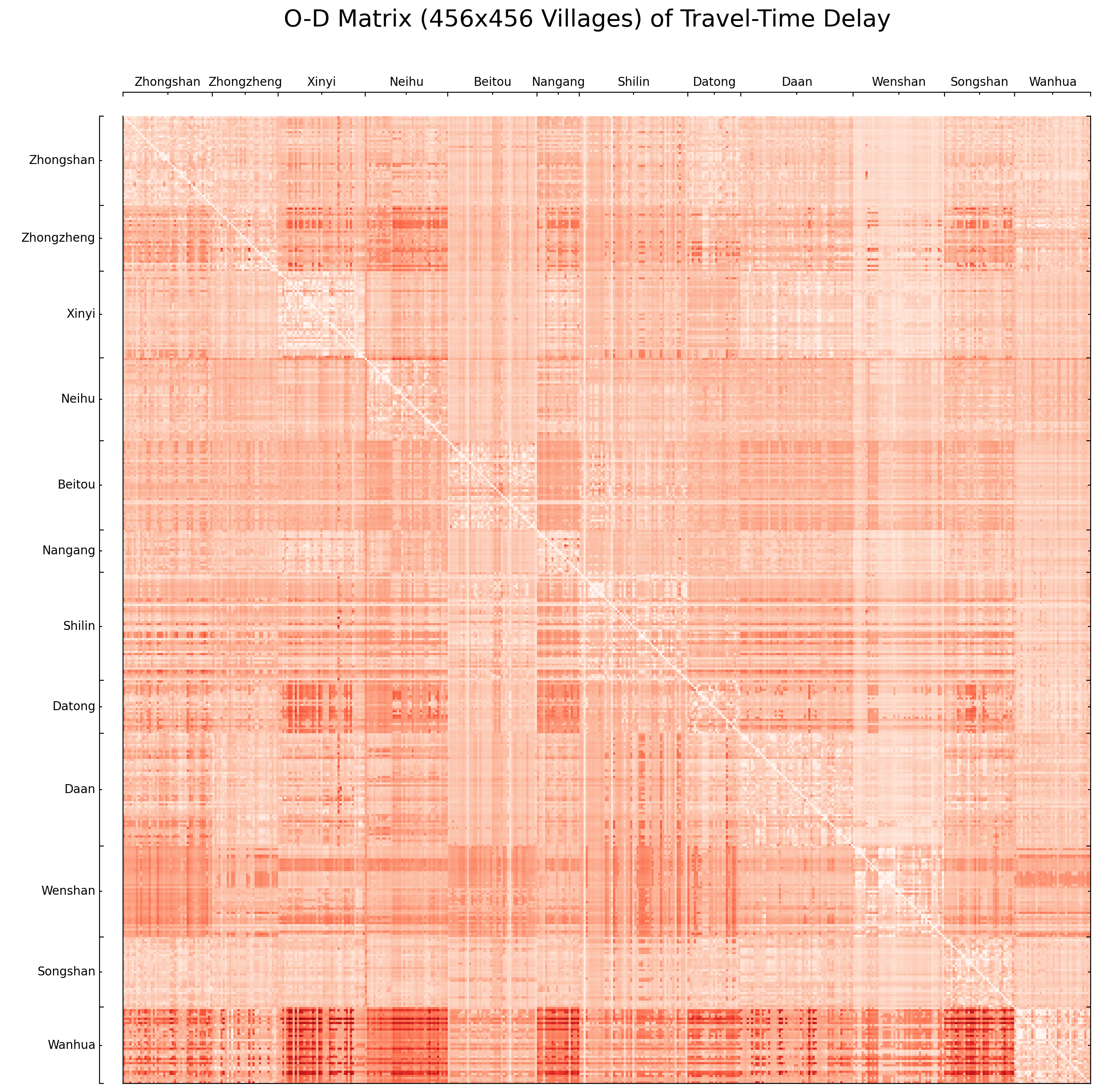
Convert the 207,936 data points to a 456x456 pivot table results the origin-destination matrix, as visualized in below image. Each row represents the travel-time delay of 456 routes originated from one specific village, and similarly each column represents the delay destined to one village. The darker the color, the worse the delay. The x and y label are the districts, the upper administrative subdivision above villages. It is obvious that some districts have worse traffic condition than others.
Travel Time Delay at the District Scale
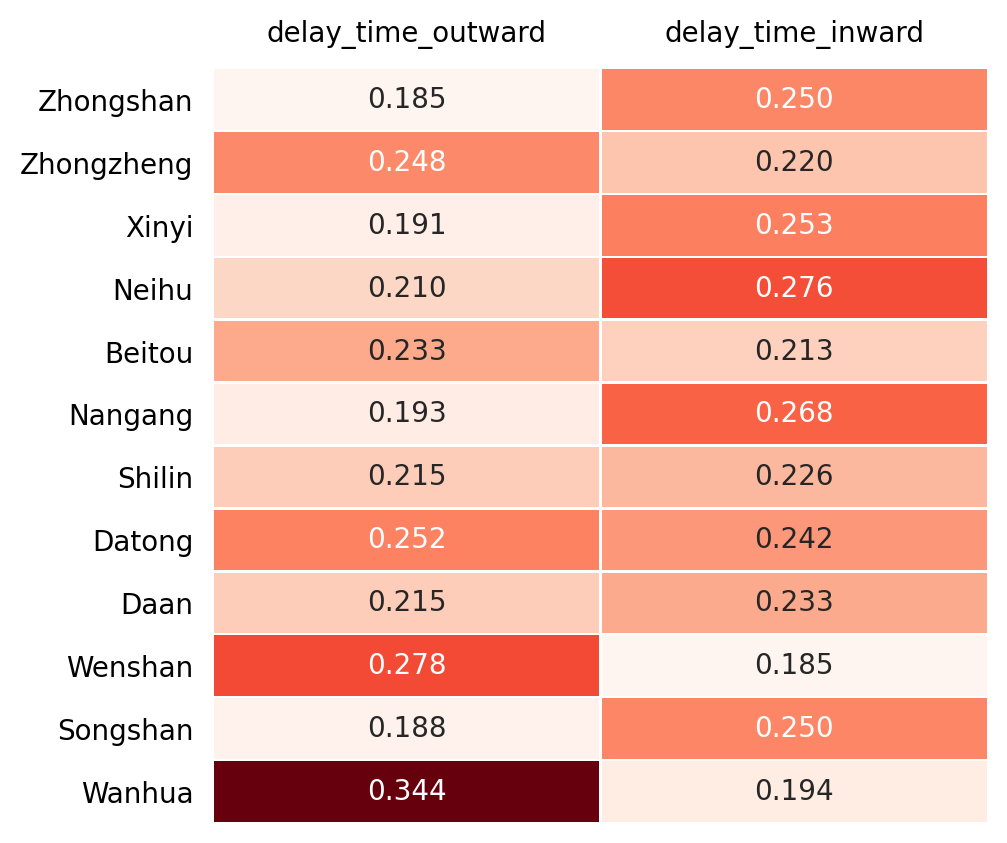
Zooming out the O-D matrix to district scale gives a clearer idea about the traffic conditions, as shown in below figure. Routes originated from Wanhua have much worse travel-time delay than the rest, followed by Wenshan and Datong districts. However the story is complete different in the opposite direction. As the destination, Wenshan and Wanhua are the least delayed, while Neihu and Nangang are the worst.
More specifically, the worst traffic happens in the routes between Wanhua and Neihu (45.0% of travel-time delay), Wanhua and Songshan (44.9%), and Wanhua and Nangang (44.8%).
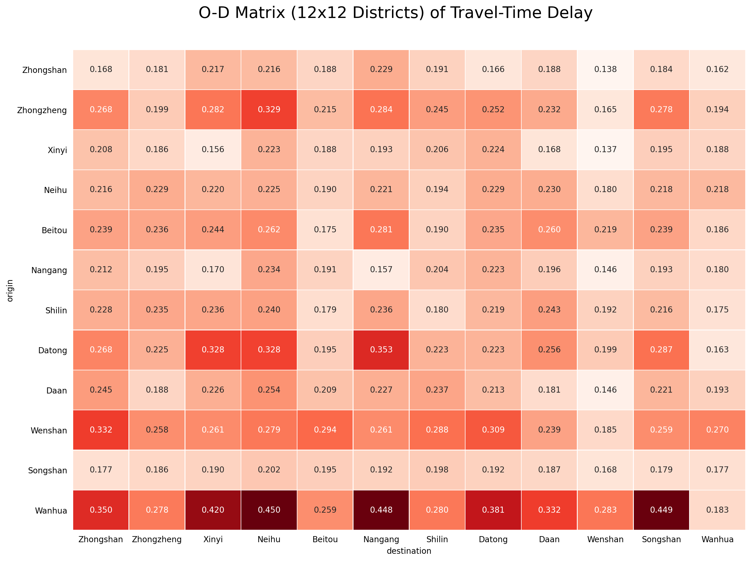
Below table shows the average travel-time delay of each district as both the origin (outward) and the destination (inward).
TRAVEL-TIME DELAY OF VILLAGES
The average departure (outward) travel-time delay of each village takes into account all the routes originated from one specific village to other 455 villages. It is calculated by first summing up both base time and traffic time respectively (note that this result is NOT the same as simply taking the mean value of all routes’ delay). Likewise, the average arrival (inward) travel-time delay of each village is derived.
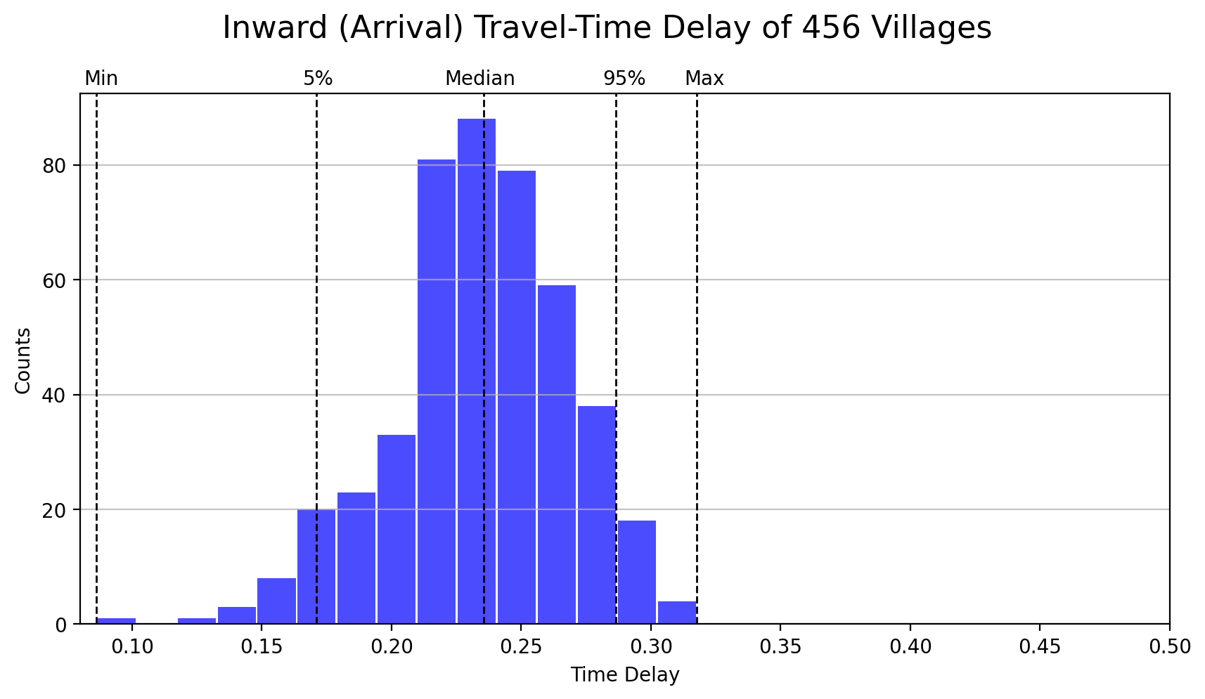
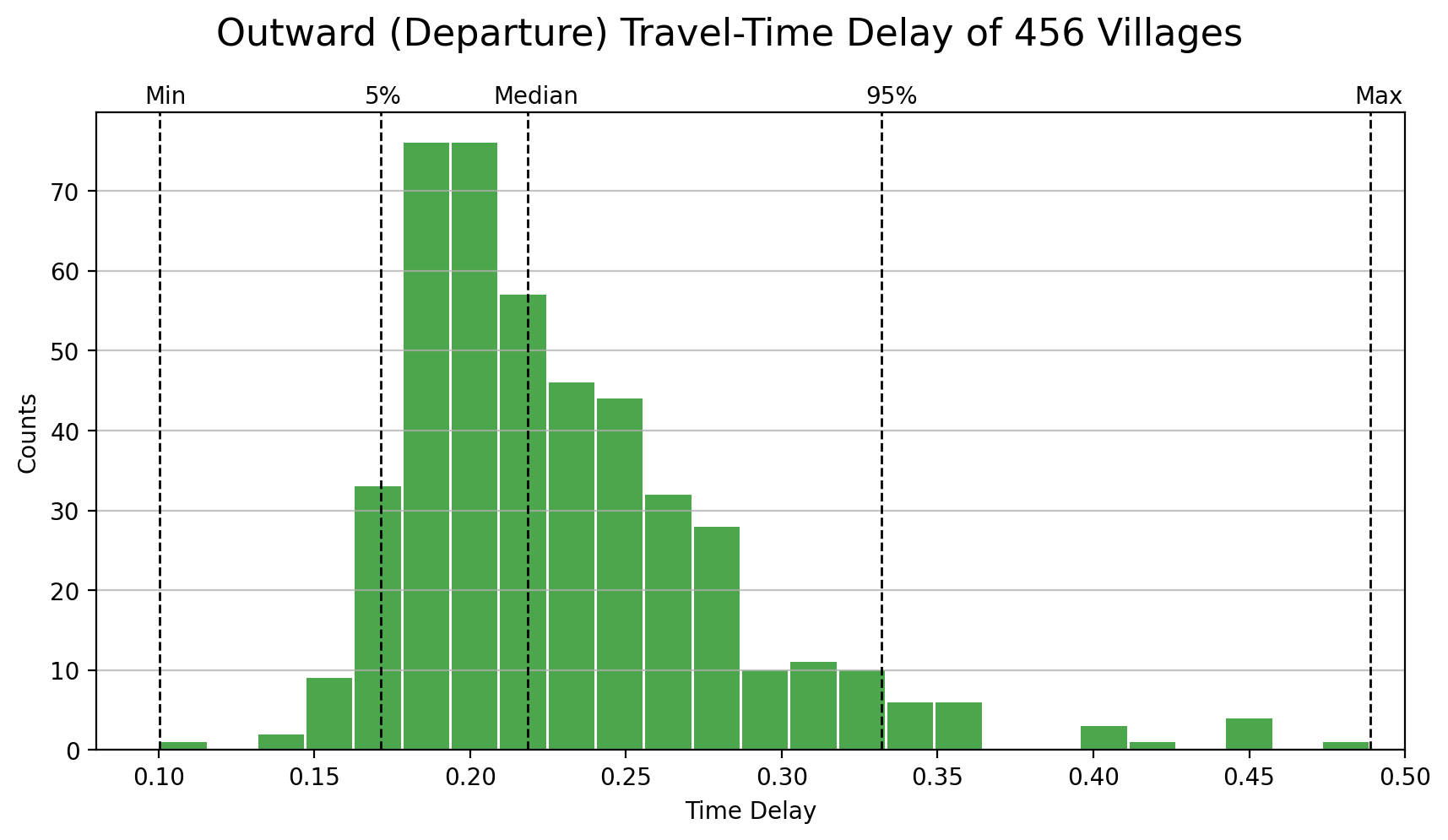
Below two figures show the distribution of inward and outward delay of 456 villages respectively. Most villages have inward travel time delay between 0.17 and 0.28, that is, the traffic time to arrive at each village is about 17% to 28% longer than base time. The outward delay of most villages is between 17% and 33%.
The biggest difference between these two figures is that the distribution of inward delay is left-skewed and outward delay is right-skewed. In other words, some villages, as the origin, have much worse traffic conditions than average.
Where are they?
The two interactive maps below show the travel-time delay of the 456 villages as both the destination and the origin, separately. The darker and taller prisms have worse delay time.
First look at the map of inward delay. It is clear that the worse villages concentrate in the east part of the City, which belongs to Neihu and Nangang districts, as also found in the previous section. These two districts host the major software and technology park with massive employment, which explains the arrival travel-time delay during the morning rush hours. It also implies the insufficient transportation infrastructure in this area.
Similar to the findings from the O-D matrix in the last section, districts including Wanhua, Wenshan, Datong and Zhongzheng have worse outward traffic condition as the origin of the routes. However, what is interesting here is the distribution of the worse villages within these districts.
While the villages with worse inward travel-time delay form a cluster in Neihu and Nangang, those with worse outward delay show a ribbon-like distribution along the western border of Taipei City. The reason that causes this is completely different. The truth is that these villages are gateways of the City. Every morning lots of trips originated from the suburbs enter the City (mostly through bridges), which leads to the terrible traffic congestion and travel-time delay.
TRAVEL-TIME DELAY OF EDGES
Finally let’s look at the edges that exist in real world. In Part III, 2,070 edges that connect the 456 nodes and therefore the entire network are identified. The average travel-time delay of these edges are then to be calculated, visualized and discussed in this section.
The average travel-time delay of each edge is calculated as follows:
- Find out all routes that contain the specific edge;
- Summing up separately the base time and traffic time of these routes; and
- Calculate the average travel-time delay.
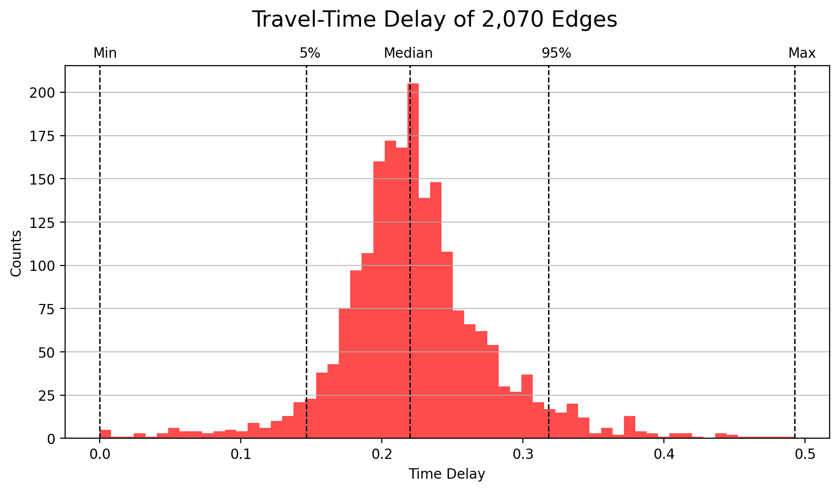
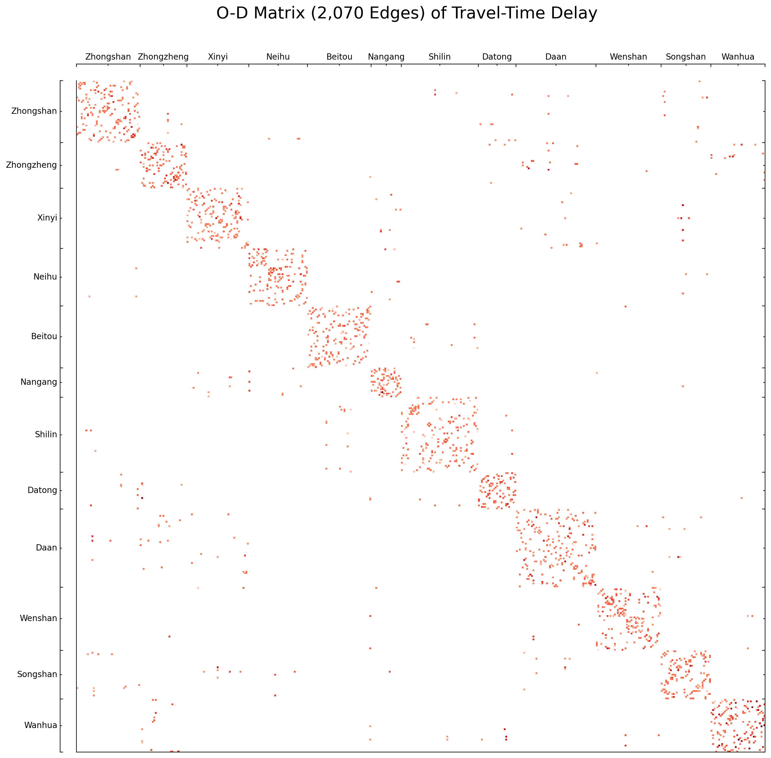
Below two figures are the frequency distribution and O-D matrix of these 2,070 edges. The travel-time delay of most edges (90%) are between 0.146 and 0.318, that is, 14.6% and 31.8% of traffic delay, while the worst delay reaches almost 50%.
Where are they?
The edges are directional but, unlike the villages, the travel-time delay of edges cannot simply be classified as inward and outward delays. To simplify the problem, the delay of each edge is averaged with its own reverse. This method has its limitation such as neglecting the different number of routes from opposite directions and the route choices. As a result, please note that it is used only for the purpose of visualization here.
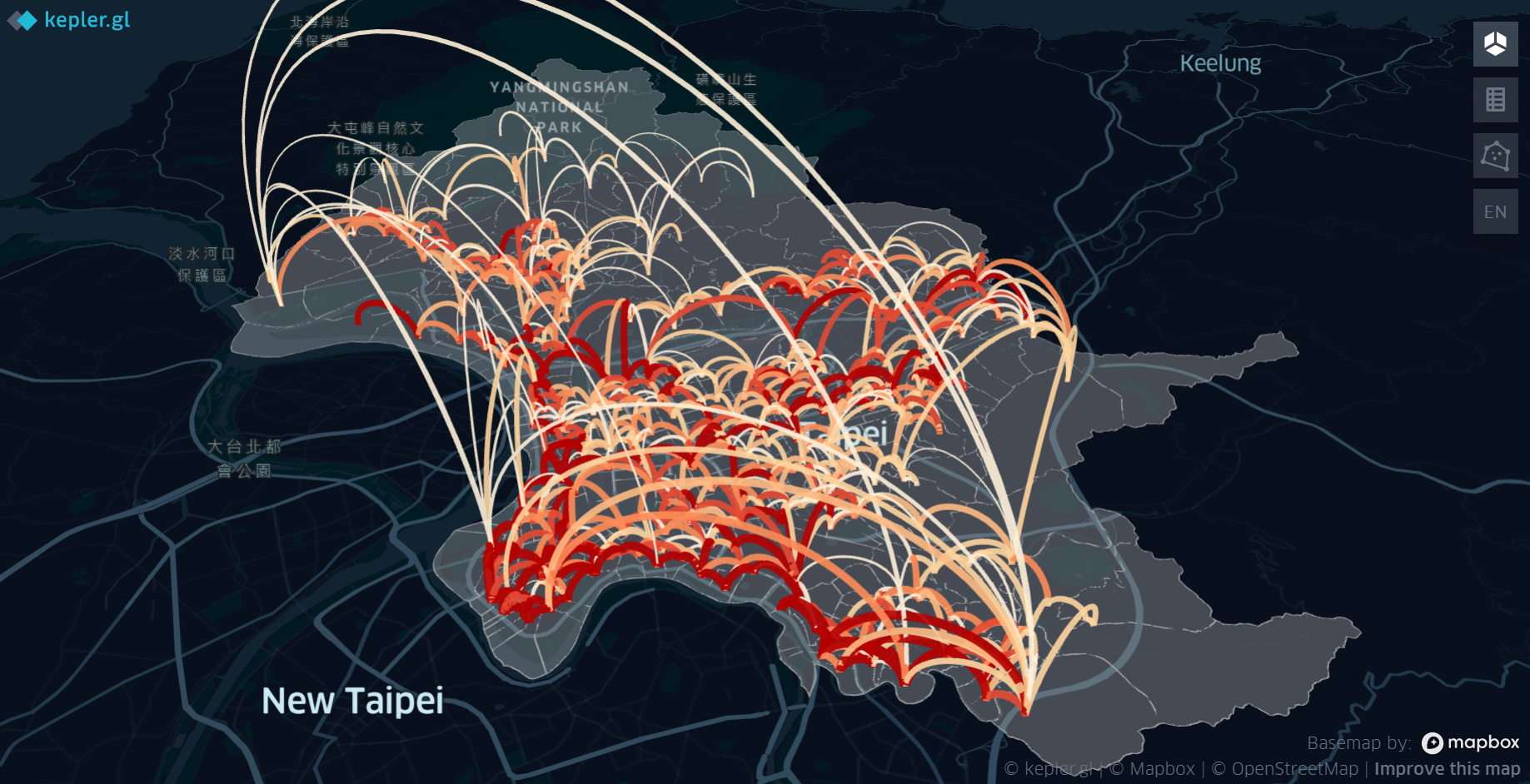
Below map illustrates these edges (represented by arcs) and their travel-time delay. The delay gets worse when the arcs gets darker and thicker.
The result confirms what’s found from the delay of villages in the previous section. The edges from the eastern part of the City (Neihu, Nangang) and along the western border (Wanhua, Wenshan, Datong) have relatively bad traffic conditions. In addition, there seems to exist two parallel corridors connecting the east and the west, which consist of edges with worse travel-time delay. This is an interesting finding, which implies and reinforces the flow of the traffic during the morning rush hours.
SUMMARY OF PART IV-(1)
In this post, the travel-time delay of all 207,936 routes, 456 villages and 2,070 edges within the network of the City is calculated, visualized and discussed. Using the traffic data acquired from HERE Routing API, this study identifies the villages as well as the edges with relatively bad traffic condition during morning peak time.
In the next and last post of this series of study, the employment as well as the residents of the villages will be taken into consideration, serving as the pull and push force of the traffic flow. Finally, by integrating the findings of betweenness (as the probability of network usage), the travel-time delay (as the indicator to the sufficiency of infrastructure) and the nodes’ weights (as the demand and supply of the traffic flow), this study will conclude and identify the key zones in need of the immediately improvement.
SOURCE CODES
All source codes used in this post can be found on Colab or my GitHub.
INDEX