PART III-(2) OF THE REPRESENTATION AND MEASUREMENTS OF URBAN TRANSPORTATION NETWORKS
In this post I examine the betweenness centrality of 456 nodes and 2070 edges in the real world transportation network, and identify the potential high-risk traffic zones. Unlike closeness centrality which represents the accessibility of the nodes, betweenness measures the probability of the nodes/edges being used while travelling in the City. In other words, when a node/edge with high betweenness score is removed (blocked), a great number of routes will be affected.
PREVIOUSLY ON THE REPRESENTATION AND MEASUREMENTS OF URBAN TRANSPORTATION NETWORKS
In Part III of this study, the SNA approach is adopted for the analysis of the weighted, directed transportation network of the real world. The previous post looks at the closeness centrality of the network and identifies the most accessible nodes within it. Such nodes have relatively shorter travel time to/from all other nodes and therefore become a good choice as a logistics distribution/collection center. By taking the villages’ population as nodes’ weight into consideration, the previous post also discusses the service coverage problem.
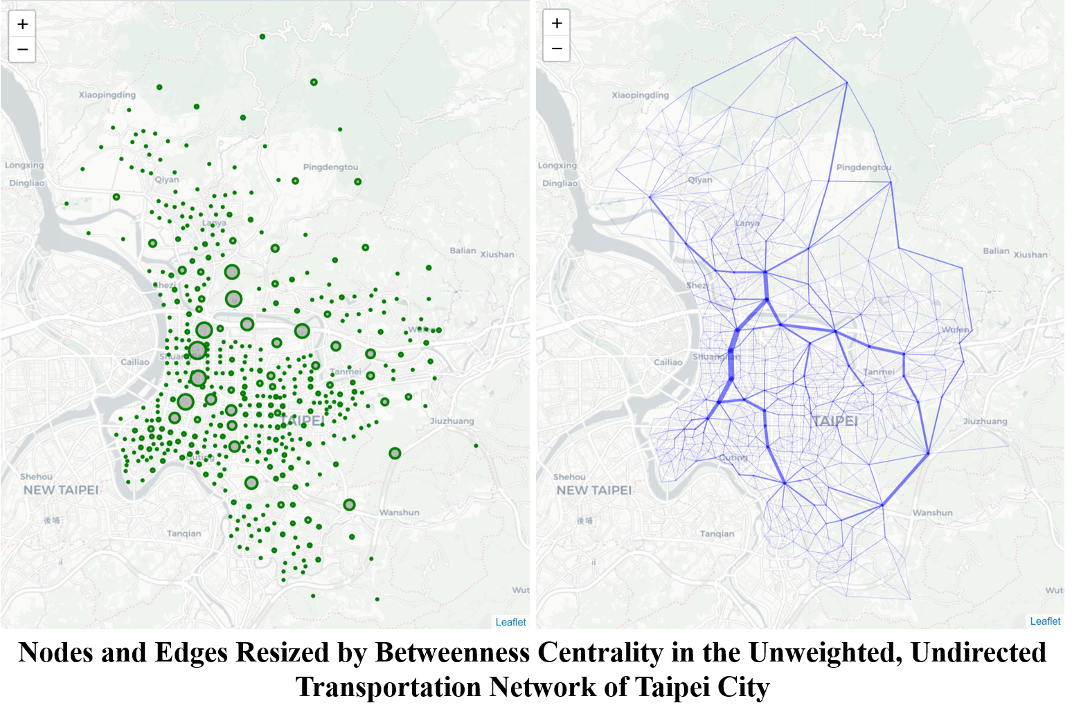
This post continues with the second important SNA measurement – betweenness centrality. Below images show the findings in Part I of the study for betweenness scores of both nodes (left) and edges (right) in the unweighted and undirected network. In both images there seems to exist some mainstreams where smaller branches flow into. The mainstreams consist of higher-score nodes and edges, providing a shorter path between two random nodes in the network. This post will also examine whether such mainstreams are in place or not.
THE DEFINITION OF BETWEENNESS CENTRALITY IN REAL WORLD
Simply put, the betweenness centrality of a node is the probability of passing through that node while travelling in the network. Take the 456 nodes of the Taipei City network for example: counting the 455 routes to all other nodes originated from each node amounts to 456x455 different routes (note that these are directed routes so that the route from node A to B is not equal to that from B to A); and a node’s betweenness centrality is the percentage of the 456x455 routes using that node.
More specifically, the betweenness centrality of a node is defined as:
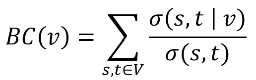
where BC(v) is the betweenness centrality of node v; σ(s,t) is the number of all shortest paths from node s to node t; σ(s,t|v) is the number of these shortest paths that pass through node v; and node s, t, v belong to the same network V where s≠t≠v.
Theoretically there could be more than one shortest path between any two nodes. Assume that 5 shortest paths exist between node s and t, where only 2 of them pass through v. The probability of v being used is then 0.4. In this study, the betweenness of node v is calculated by first summing up all these probabilities between all pairs of nodes (s,t), which are then divided by 456x455 for normalization. The final score is the probability of node v being used in all shortest paths.
Similarly, the edge betweenness centrality of an edge is the likelihood of the edge being used while moving in the network, defined as:
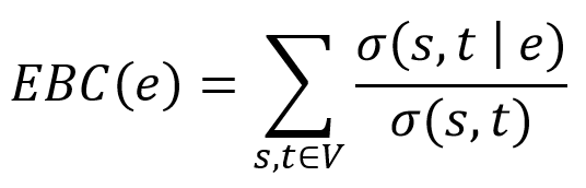
where EBC(e) is the edge betweenness centrality of edge e; and σ(s,t|e) is the number of shortest paths between node s and t that pass through e where s≠t.
This study will measure and discuss the betweenness centrality of both nodes and edges, respectively.
DATA
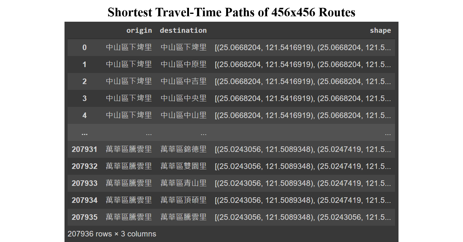
In Part II of this study, HERE Routing API is used to request the shortest (travel time) paths between all pairs of the 456 village offices in Taipei City. The response of a shortest path consists of a list of coordinates, starting from the coordinate of the origin node and ending at that of the destination. Below image shows an example of 455 different shortest paths from one specific node to all others. The table shows all lists of the 456x456 shortest paths.
CONVERTING ROUTE SHAPES TO LISTS OF NODES
Before continuing to the centrality calculation, these lists of paths consisting of coordinates have to be converted to lists of nodes and edges. Here different algorithms have been created and revised for the conversion and discussed below.
Algorithm 0
First this study tries to convert each route list by simply identifying the villages where the coordinates within the list locate. Specifically speaking,
-
Find the village polygon that contains each coordinate in the list and replace the coordinate with the node that represents the village polygon;
-
Remove duplicated nodes in a list; and
-
Revise the origin and destination if they don’t match the route.
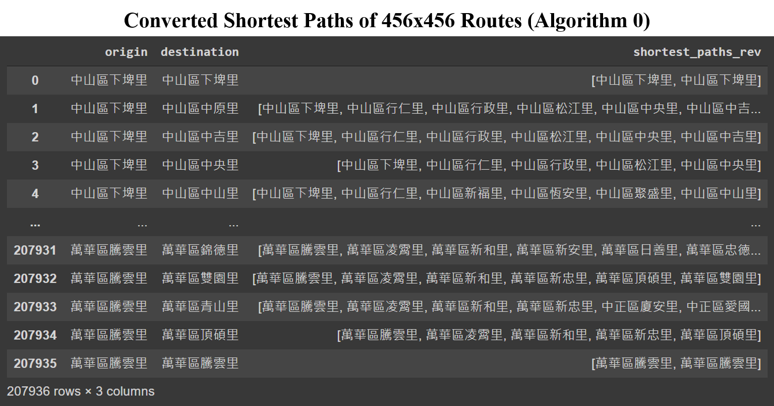
Below table shows the 207,936 (456x456) shortest paths converted from the lists of coordinates to lists of nodes.
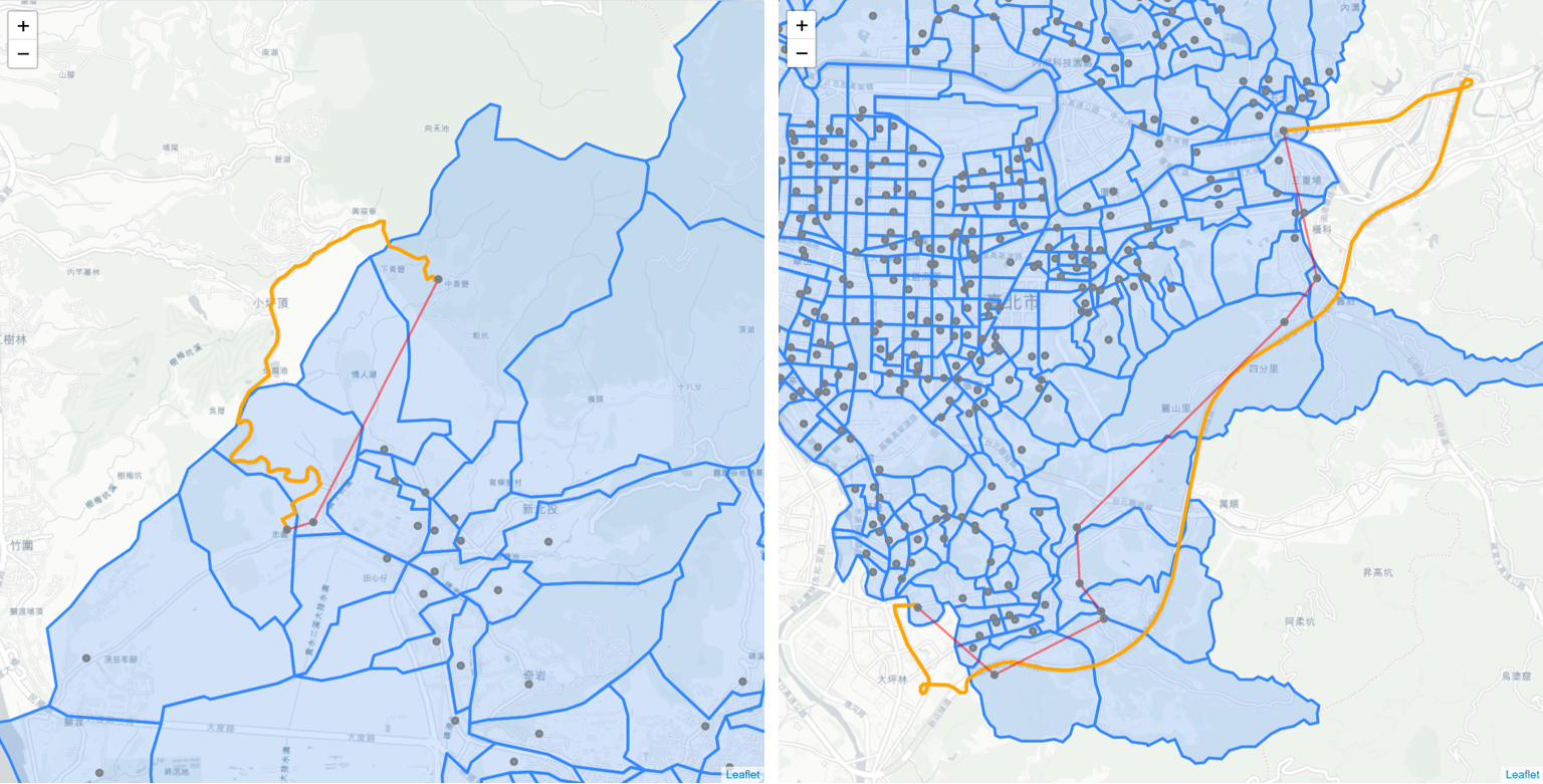
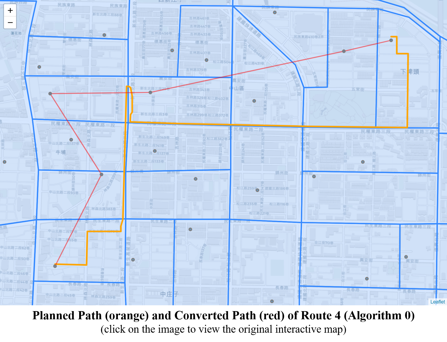
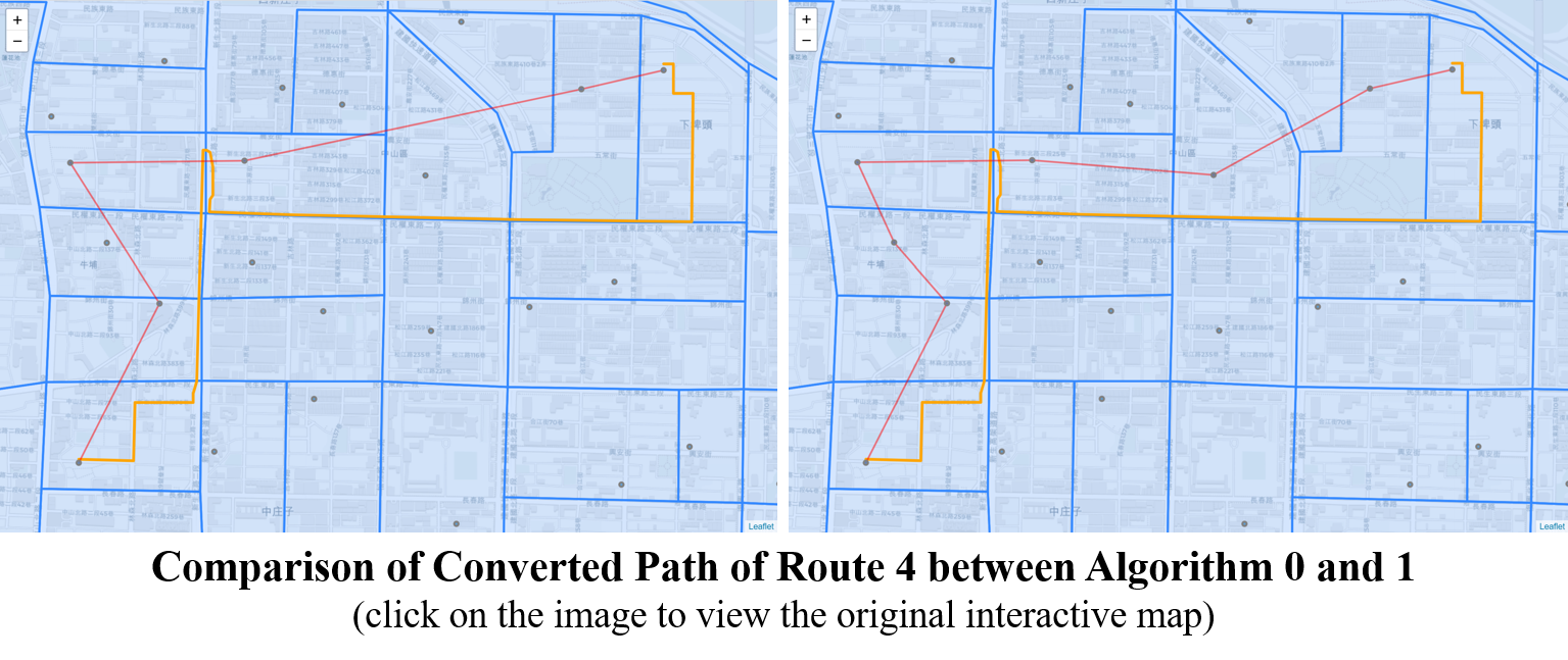
Unfortunately this algorithm is far from perfect. Below image shows route No. 4 before and after conversion, where the orange route represents the real world shortest path (consisting of coordinates) and the red route consists of nodes and edges. It is clear that in the image the red route skips two nodes along the path. The reason why they are skipped is because there are no points of coordinates (returned from HERE Routing API) locating within the skipped village polygons, given that the planned route near the area is a straight line.
As a result of missing nodes along the route, more unexpected edges are created. That is, as per its definition, an edge can only exist between two neighboring villages, and now two separated villages can be connected by jumping over the skipped node.
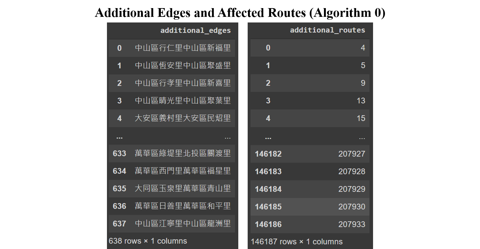
638 unique additional edges are found in 146,187 routes as shown in below tables, accounting for 70.5% of total routes. Below image shows where these additional edges are in the map.
These additional edges will significantly affect the results of the betweenness centrality, in that they decrease the probability of the original edges to be used, and they also violate the definition of edges in this study, making the network much more complicated. The next algorithms are going to fix the issue by eliminating the additional edges.
Algorithm 1
This algorithm focuses on the 146,187 routes, each contains at least one of the 638 additional edges found with Algorithm 0, and tries to prevent additional edges from being used.
-
Find all segments (each consisting of two coordinates) forming the additional edges within the 146,187 routes;
-
Divide each segment found in step 1 into 4 equal parts, which then yields 3 more coordinates, and add these 3 coordinates into the list inbetween the segment; and
-
Repeat Algorithm 0.
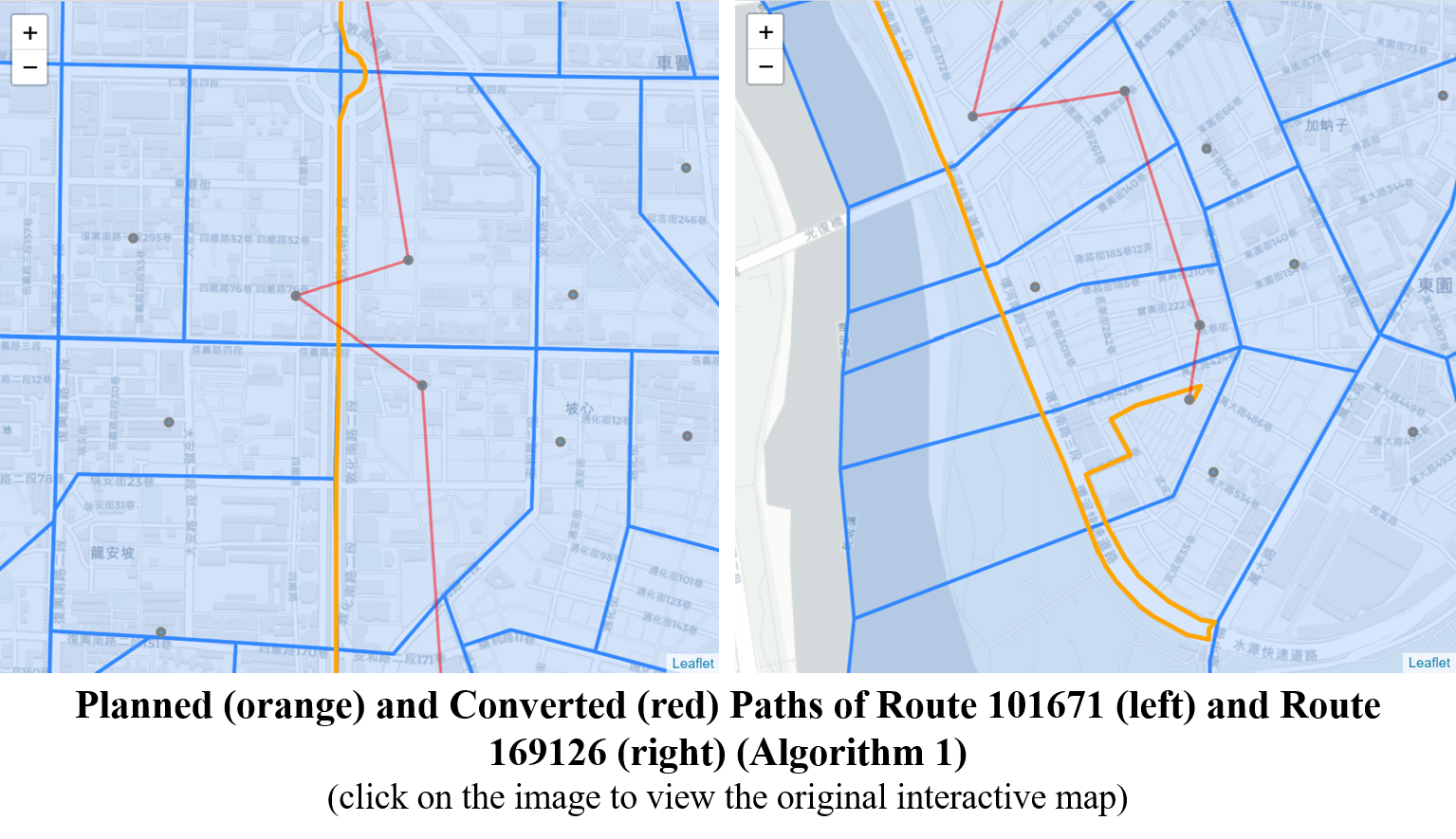
Algorithm 1 effectively resolves the issue of skipped nodes in route 4, as shown below. However, apart from that, this algorithm doesn’t contribute much. There are still 566 additional edges containing in 124,862 (60.2%) routes.
Below two images show the examples of the remaining additional edges. Take a closer look finds that these edges exist because:
- The 3 more coordinates created in the algorithm are still not contained in the skipped village polygon; or
- Many villages are bordered by roads where the planned routes could use. In some cases the routes could easily cross back and forth the borders even when they are planned to take a straight line. Since either Algorithm 0 or 1 doesn’t allow duplicated nodes in a list, some nodes appear to be skipped and additional edges created. For example, it is possible that a planned real-world route passes through nodes A, B, A, C in order. Since the algorithms prevent nodes from repeating themselves, the route will be converted to A, B, C. If node B and C are not connected, an additional edge will then be created.
Algorithm 2
This algorithm aims at solving the issues raised in the previous two algorithms:
-
Allow duplicated nodes appearing in a converted route, as long as they are not back-to-back connected;
-
Find all segments (each consisting of two coordinates) forming the additional edges within 146,187 routes;
-
Find all village polygons that intersect with each segment found in step 2 and add into the converted list of nodes; and
-
Repeat Algorithm 0.
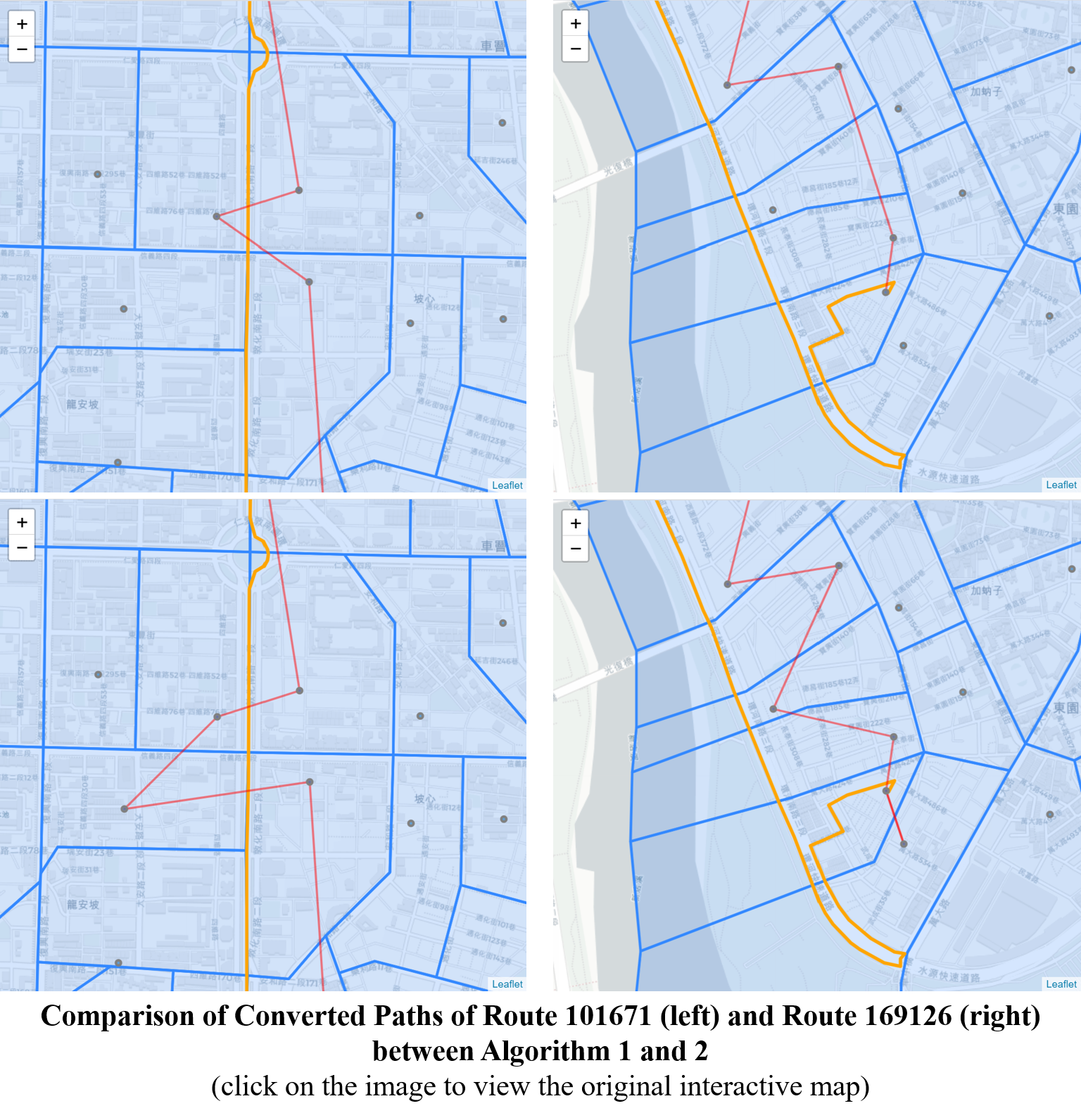
This algorithm successfully resolves the issue of additional edges in the examples shown in Algorithm 1. It also effectively reduce the additional edges from 638 to 48, and affected routes from 146,187 to 5,520, accounting for only 2.7% of all routes.
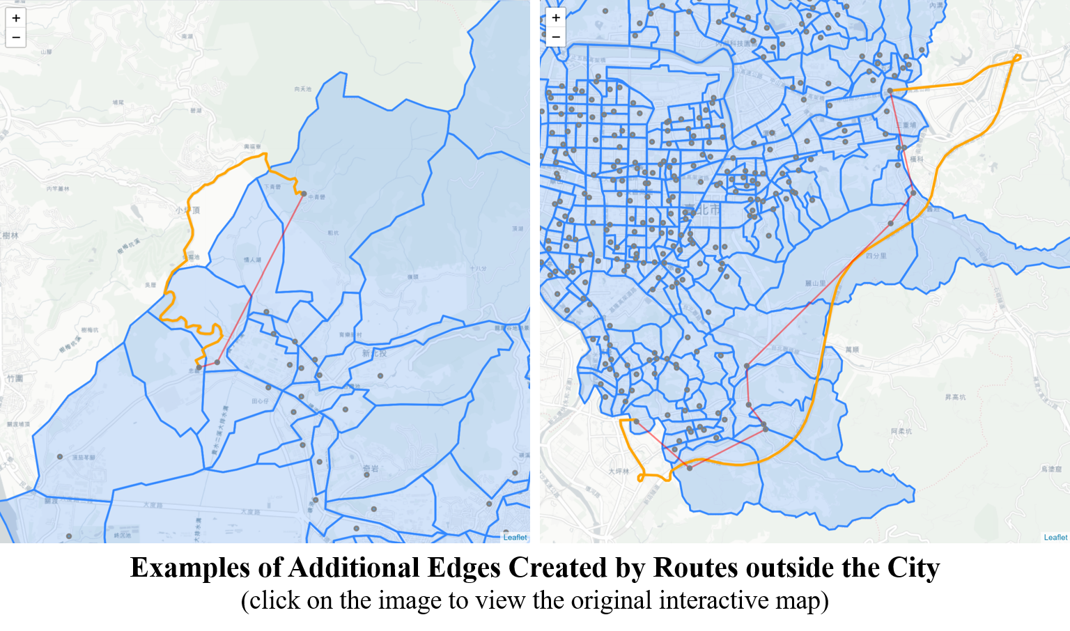
Additional Edges from Outside the Network
Below images show the comparison of additional edges derived from Algorithm 0 and 2. The additional edges that Algorithm 2 eliminates are mostly from routes within the network. The reason why there still remains 48 unique edges is that the routes take place from outside the City. Because of the shape of the City and the existence of express ways, two peripheral villages may connect with each other faster through a route beyond the City.
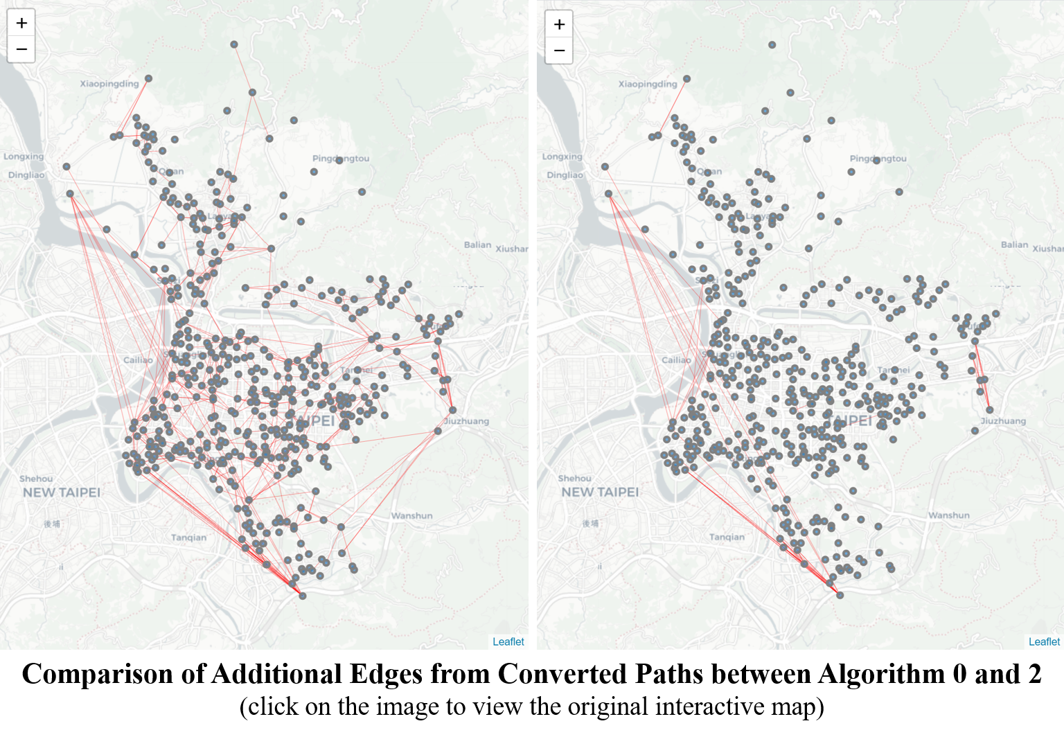
Given that the focus of this study is to identify the potential traffic conflict areas in the City, the shortest paths shall reflect the actual choice of travelling, even if they may use some routes outside the City. This simply implies that such traffic will not impact the traffic within the City.
RESULTS
Nodes Betweenness
After converting the 456x455 routes into lists of nodes and edges, this study can finally proceed to calculate the betweenness centrality. Please note that even though duplicated nodes are allowed in the routes to prevent additional edges, each node shall still be counted only once in one single route.
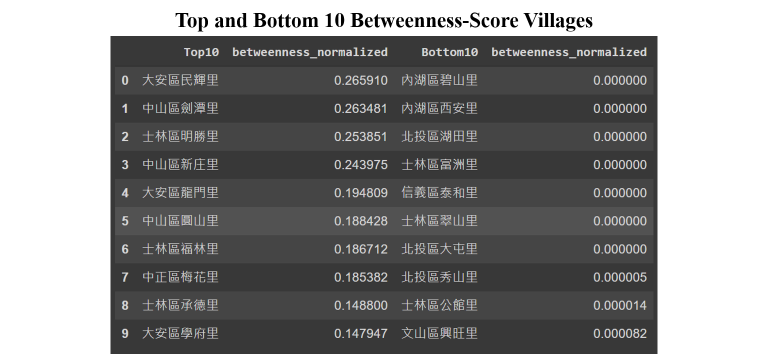
Below table shows the results of the top and bottom 10 villages and their betweenness scores. The top village has the score of 0.265910, meaning that it appears in more than a quarter of the total 456x455 routes. In the opposite, there are seven villages scored zero. In other words, except of being an origin or destination, these villages will never be used while travelling in the City.
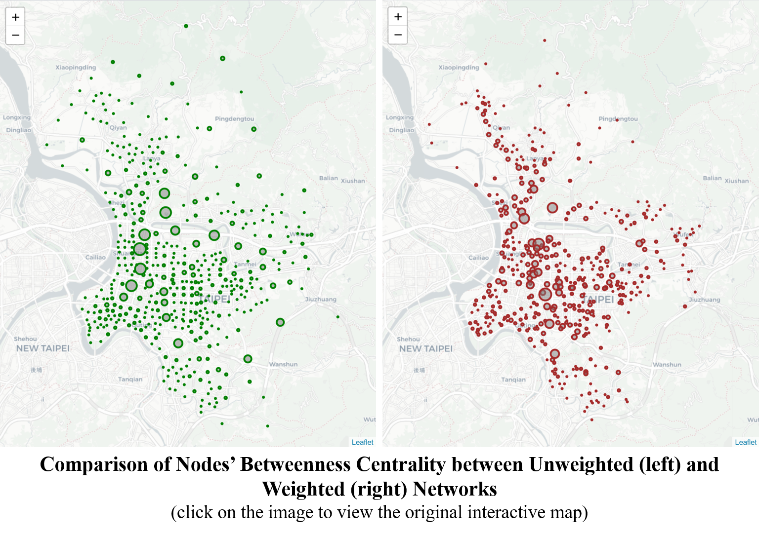
Below images show the comparison between unweighted and weighted networks with nodes resized by the betweenness scores. Similar to what is shown in the unweighted network, there also seems to be mainstreams connecting higher-score nodes. However unlike the unweighted network,
- The mainstream in the real-world network does not consist of the same nodes as those of the unweighted;
- In the unweighted network, the gap between nodes in the mainstream and others is much larger than the gap in the weighted network. That is, the choice of routes is more diverse while travelling in the real world; and
- The betweenness scores in some peripheral nodes are higher than expected in the unweighted network, implying that these nodes are used by a few routes, while in the real-world network, these nodes are simply dead ends.
Edge Betweenness
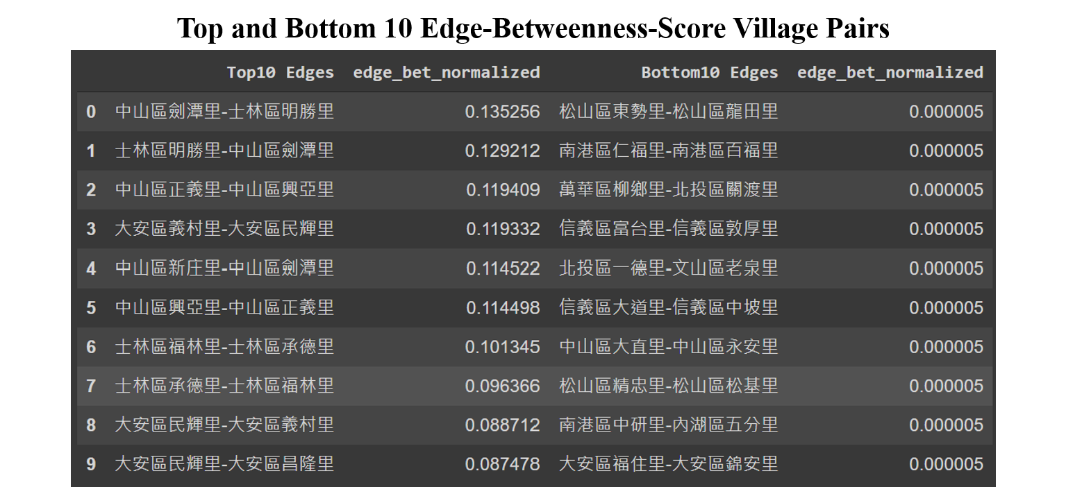
There are 2,070 unique edges found in the 456x455 routes. These edges’ betweenness centrality are then calculated. Below table shows top and bottom 10 edges and their betweenness scores.
Please note that there could be 2 different direction edges between the same pair of nodes. For example, among the top 10, edges 0 & 1 share the same two nodes in opposite direction; so does edges 2 & 5, edges 3 & 8, and edges 6 & 7. The betweenness score of the top edge reaches 0.135256, meaning that it is passed by 13.5256% of the total 456x455 routes. Similarly, all bottom 10 edges have the same score of 0.000005, which implies that these edges are used in only one route among more than 200K routes. However, they may still not be the least used edges since at least they appear once in the shortest paths. There could exist some edges that no one will ever travel through in the network.
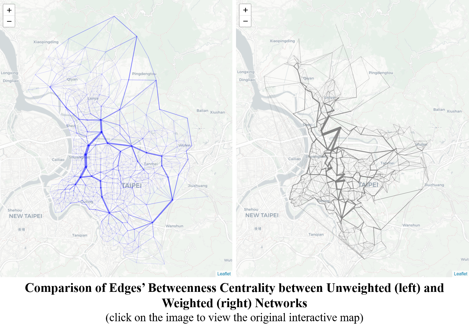
Showing below are images from both unweighted (left) and weighted (right) networks where the edges are resized by the betweenness scores. Since the edges are directional in the real-world network, the size (thickness) of the edge are represented by the edge with higher score. These two images show that:
- Similar to the findings in the previous section, there are some mainstreams connecting the up-town throughout the down-town;
- The mainstreams shown in the unweighted network creates a clear hierarchy above other edges. However such hierarchy is rather vague in the real-world network. There does not exist one single route that collects all branches, which implies that the choice of routing is much more flexible; and
- The edges connecting eastern peripheral nodes do not exist.
Below image shows the nodes and edges both resized by their betweenness scores at the same time.
Redundant Edges
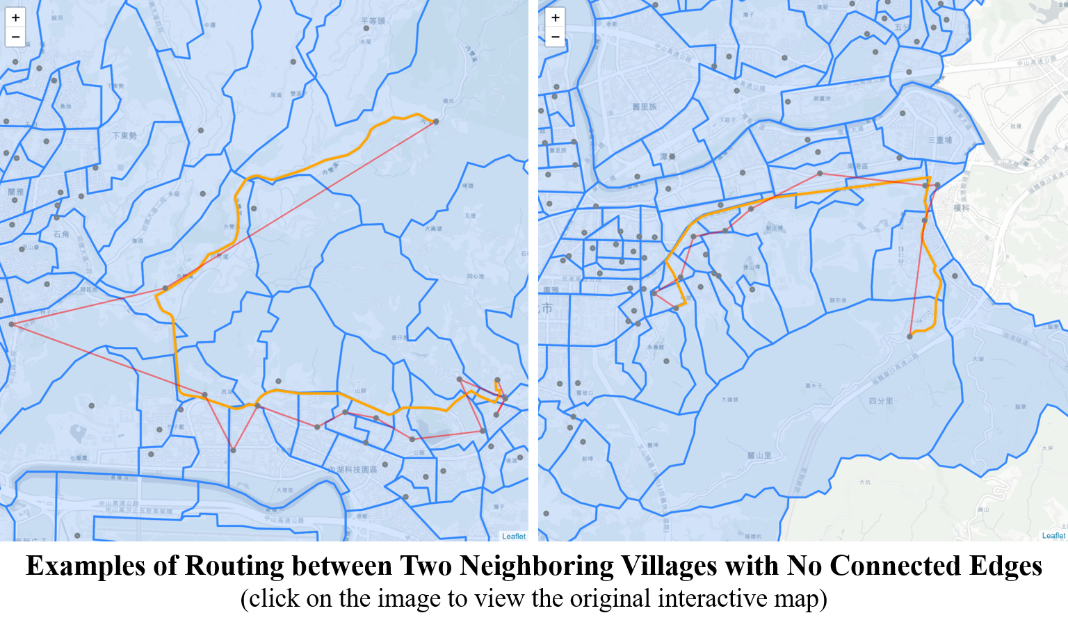
In Part I of the study, an edges between two nodes in the unweighted network is created as long as the village polygons share the border. In real-world transportation network, some of these created edges may just never be used in any shortest paths.
Comparing the edges created in the unweighted network with edges used in the weighted, directed network shows that 352 edges in the unweighted network are not used in the real world. In other words, there are 352 pairs of neighboring villages connected through a third one.
Below image shows these edges on the map. The reason why the direct routes are not the shortest paths could be that these routes are traffic detours or they simply don’t exist. Such occasions happen in the peripheral hilly areas, or between villages separated by rivers, military bases or the airport.
SUMMARY OF PART III (2)
This post examines the betweenness centrality of both nodes and edges in the real world. Unlike closeness centrality which represents the accessibility of the nodes, betweenness measures the probability of the nodes/edges being used while travelling in the network. In other words, when a node/edge with high betweenness score is removed (blocked), a great number of paths will be affected. Such node/edge could become the critical traffic zone in the transportation network.
Having said that, betweenness centrality can only measure the probability and has its limitation, such as:
- The probability could change significantly when taking weights of nodes into consideration. For example, the highest betweenness score of nodes in this post is about 0.26, meaning the node will be used in 26% of the routes. Assume that all origins and destinations included in these routes only account for 1% of the City’s population while 99% distribute in the rest of the villages. Under such extreme condition, the node with the highest betweenness score may not need any further attention.
- The traffic condition between peak and off-peak hours is not considered. It is hard to tell which of the followings needs immediate improvement: an edge with the highest betweenness score and 5% travel-time delay in rush hours, or another edge ranked 51st in betweenness but 500% worse in traffic time during rush hours.
In Part IV, the weights of nodes as well as the traffic time difference between peak and off-peak hours will be introduced to identify the potential high-risk areas.
SOURCE CODES
All source codes used in this post can be found on Colab or my GitHub.
INDEX